

8.2 Basics of Diffusion
255
8.2.2 Random Walks
As we mentioned above, particles which undergo diffusion spread in space in
a very irregular manner. This is known as a random walk through space.
In 1826, a botanist, Robert Brown observed with the aid of a microscope,
an irregular motion performed by small particles of colloidal size immersed in
a fluid which can serve as an example of random walk. The nature of these
motions remained a puzzle until the beginning of our century when Albert Einstein showed that this 'Brownian motion' is maintained by collisions with the
molecules of the surrounding fluid. During each collision, a randomly oriented
impulse on the particle results in their spreading. Statistical analysis of Brownian motion is a starting point for an attack on the more difficult problems of
diffusion. Therefore, for better understanding of the random walk, following
Okubo (1980), we will consider a simple case of particles which can spread
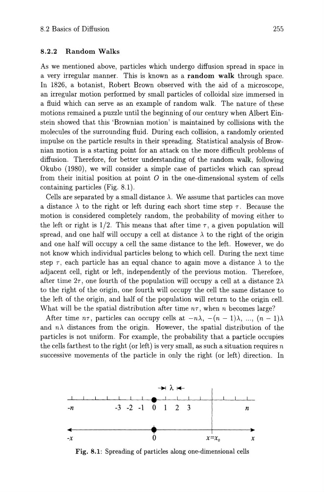
from their initial position at point 0 in the one-dimensional system of cells
containing particles (Fig. 8.1).
Cells are separated by a small distance'\. We assume that particles can move
a distance ,\ to the right or left during each short time step T. Because the
motion is considered completely random, the probability of moving either to
the left or right is 1/2. This means that after time T, a given population will
spread, and one half will occupy a cell at distance ,\ to the right of the origin
and one half will occupy a cell the same distance to the left. However, we do
not know which individual particles belong to which cell. During the next time
step T, each particle has an equal chance to again move a distance ,\ to the
adjacent cell, right or left, independently of the previous motion. Therefore,
after time 2T, one fourth of the population will occupy a cell at a distance 2,\
to the right of the origin, one fourth will occupy the cell the same distance to
the left of the origin, and half of the population will return to the origin cell.
What will be the spatial distribution after time nT, when n becomes large?
After time nT, particles can occupy cells at -n'\, -(n - 1),\, ... , (n - 1)'\
and n'\ distances from the origin. However, the spatial distribution of the
particles is not uniform. For example, the probability that a particle occupies
the cells farthest to the right (or left) is very small, as such a situation requires n
successive movements of the particle in only the right (or left) direction. In
-n
-3 -2 -1 0
2 3
n
-x
o
x
Fig. 8.1: Spreading of particles along one-dimensional cells
255
8.2.2 Random Walks
As we mentioned above, particles which undergo diffusion spread in space in
a very irregular manner. This is known as a random walk through space.
In 1826, a botanist, Robert Brown observed with the aid of a microscope,
an irregular motion performed by small particles of colloidal size immersed in
a fluid which can serve as an example of random walk. The nature of these
motions remained a puzzle until the beginning of our century when Albert Einstein showed that this 'Brownian motion' is maintained by collisions with the
molecules of the surrounding fluid. During each collision, a randomly oriented
impulse on the particle results in their spreading. Statistical analysis of Brownian motion is a starting point for an attack on the more difficult problems of
diffusion. Therefore, for better understanding of the random walk, following
Okubo (1980), we will consider a simple case of particles which can spread
from their initial position at point 0 in the one-dimensional system of cells
containing particles (Fig. 8.1).
Cells are separated by a small distance'\. We assume that particles can move
a distance ,\ to the right or left during each short time step T. Because the
motion is considered completely random, the probability of moving either to
the left or right is 1/2. This means that after time T, a given population will
spread, and one half will occupy a cell at distance ,\ to the right of the origin
and one half will occupy a cell the same distance to the left. However, we do
not know which individual particles belong to which cell. During the next time
step T, each particle has an equal chance to again move a distance ,\ to the
adjacent cell, right or left, independently of the previous motion. Therefore,
after time 2T, one fourth of the population will occupy a cell at a distance 2,\
to the right of the origin, one fourth will occupy the cell the same distance to
the left of the origin, and half of the population will return to the origin cell.
What will be the spatial distribution after time nT, when n becomes large?
After time nT, particles can occupy cells at -n'\, -(n - 1),\, ... , (n - 1)'\
and n'\ distances from the origin. However, the spatial distribution of the
particles is not uniform. For example, the probability that a particle occupies
the cells farthest to the right (or left) is very small, as such a situation requires n
successive movements of the particle in only the right (or left) direction. In
-n
-3 -2 -1 0
2 3
n
-x
o
x
Fig. 8.1: Spreading of particles along one-dimensional cells