

144
4 How to Determine Wave Parameters
Ot 1.0
"~~
6 "- 0.8
~
6 "- '+-..,
0.6
0.4
-2.0
-1.5
-1.0
-0.5
0.0
0.5
1.0
1.5
2.0
Displacement s (m)
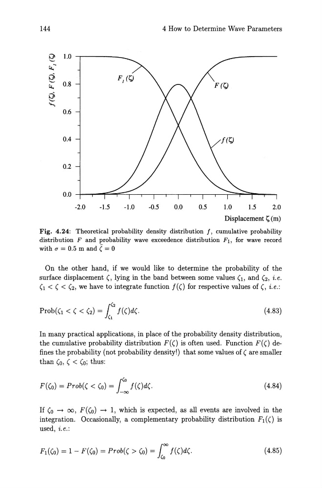
Fig. 4.24: Theoretical probability density distribution f, cumulative probability
distribution F and probability wave exceedence distribution F1, for wave record
with (J = 0.5 m and ( = 0
On the other hand, if we would like to determine the probability of the
surface displacement (, lying in the band between some values (1, and (2, i. e.
(1 < ( < (2, we have to integrate function f(() for respective values of (, i.e.:
(4.83)
In many practical applications, in place of the probability density distribution,
the cumulative probability distribution F(() is often used. Function F(() defines the probability (not probability density!) that some values of ( are smaller
than (0, ( < (0; thus:
1
<0
F((o) = Prob(( < (0) = -00 f(()d(.
(4.84)
If (0 -+ 00, F((o) -+ 1, which is expected, as all events are involved in the
integration. Occasionally, a complementary probability distribution F1 (() is
used, i.e.:
F1((0) = 1 - F((o) = Prob(( > (0) = roo f(()d(.
i(o
(4.85)
4 How to Determine Wave Parameters
Ot 1.0
"~~
6 "- 0.8
~
6 "- '+-..,
0.6
0.4
-2.0
-1.5
-1.0
-0.5
0.0
0.5
1.0
1.5
2.0
Displacement s (m)
Fig. 4.24: Theoretical probability density distribution f, cumulative probability
distribution F and probability wave exceedence distribution F1, for wave record
with (J = 0.5 m and ( = 0
On the other hand, if we would like to determine the probability of the
surface displacement (, lying in the band between some values (1, and (2, i. e.
(1 < ( < (2, we have to integrate function f(() for respective values of (, i.e.:
(4.83)
In many practical applications, in place of the probability density distribution,
the cumulative probability distribution F(() is often used. Function F(() defines the probability (not probability density!) that some values of ( are smaller
than (0, ( < (0; thus:
1
<0
F((o) = Prob(( < (0) = -00 f(()d(.
(4.84)
If (0 -+ 00, F((o) -+ 1, which is expected, as all events are involved in the
integration. Occasionally, a complementary probability distribution F1 (() is
used, i.e.:
F1((0) = 1 - F((o) = Prob(( > (0) = roo f(()d(.
i(o
(4.85)