

4.2 Wave Parameters Based on Small Amplitude Wave Theory
139
,.-...
12
S
E- II
S 10
0
t:!
0
9
..0
<:
8
'"
S 7
0
6
()
~
5
....
'"
is 4
3
2
0
0.00
0.02
0.04
0.06
0.08
0.10
0.12
Net transport velocity (m/s)
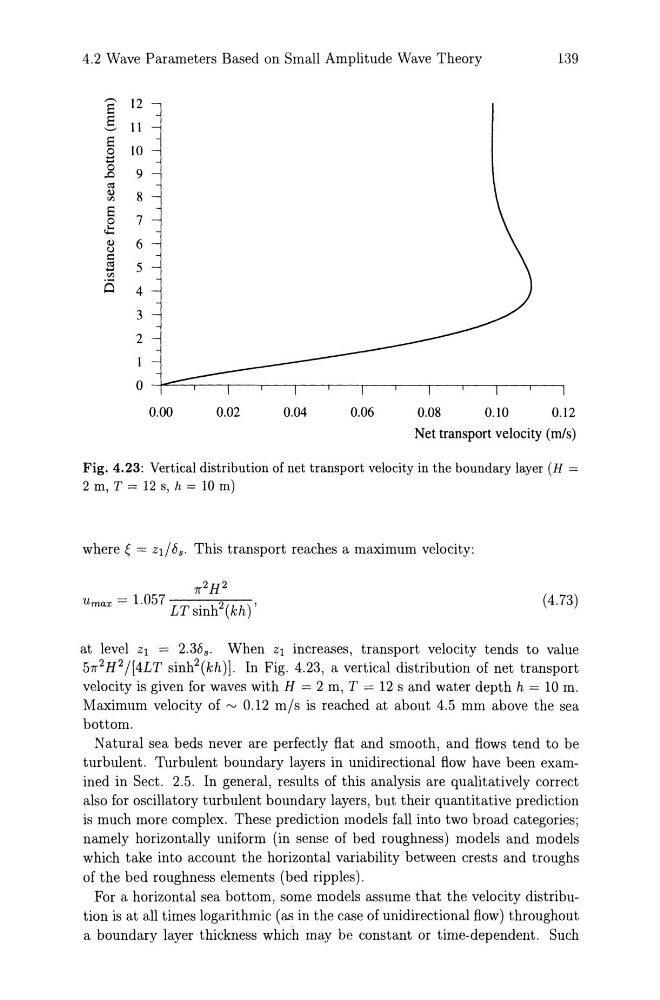
Fig. 4.23: Vertical distribution of net transport velocity in the boundary layer (H =
2 m, T = 12 s, h = 10 m)
where ~ = zd88 • This transport reaches a maximum velocity:
(4.73)
at level Zl = 2.388 , When Zl increases, transport velocity tends to value
57r 2 H2 1[4LT sinh2(kh )]. In Fig. 4.23, a vertical distribution of net transport
velocity is given for waves with H = 2 m, T = 12 s and water depth h = 10 m.
Maximum velocity of rv 0.12 mls is reached at about 4.5 mm above the sea
bottom.
Natural sea beds never are perfectly flat and smooth, and flows tend to be
turbulent. Turbulent boundary layers in unidirectional flow have been examined in Sect. 2.5. In general, results of this analysis are qualitatively correct
also for oscillatory turbulent boundary layers, but their quantitative prediction
is much more complex. These prediction models fall into two broad categories;
namely horizontally uniform (in sense of bed roughness) models and models
which take into account the horizontal variability between crests and troughs
of the bed roughness elements (bed ripples).
For a horizontal sea bottom, some models assume that the velocity distribution is at all times logarithmic (as in the case of unidirectional flow) throughout
a boundary layer thickness which may be constant or time-dependent. Such
139
,.-...
12
S
E- II
S 10
0
t:!
0
9
..0
<:
8
'"
S 7
0
6
()
~
5
....
'"
is 4
3
2
0
0.00
0.02
0.04
0.06
0.08
0.10
0.12
Net transport velocity (m/s)
Fig. 4.23: Vertical distribution of net transport velocity in the boundary layer (H =
2 m, T = 12 s, h = 10 m)
where ~ = zd88 • This transport reaches a maximum velocity:
(4.73)
at level Zl = 2.388 , When Zl increases, transport velocity tends to value
57r 2 H2 1[4LT sinh2(kh )]. In Fig. 4.23, a vertical distribution of net transport
velocity is given for waves with H = 2 m, T = 12 s and water depth h = 10 m.
Maximum velocity of rv 0.12 mls is reached at about 4.5 mm above the sea
bottom.
Natural sea beds never are perfectly flat and smooth, and flows tend to be
turbulent. Turbulent boundary layers in unidirectional flow have been examined in Sect. 2.5. In general, results of this analysis are qualitatively correct
also for oscillatory turbulent boundary layers, but their quantitative prediction
is much more complex. These prediction models fall into two broad categories;
namely horizontally uniform (in sense of bed roughness) models and models
which take into account the horizontal variability between crests and troughs
of the bed roughness elements (bed ripples).
For a horizontal sea bottom, some models assume that the velocity distribution is at all times logarithmic (as in the case of unidirectional flow) throughout
a boundary layer thickness which may be constant or time-dependent. Such