

4.2 Wave Parameters Based on Small Amplitude Wave Theory
S:8
~7
.~ 6
~
:> 5
~
~ 4
3
2
1
solitary wave profile
small amplitude
wave profile
123
o ~==~~--~~~~~~--------~r-~~===--1
-2
-3
-4 ~'-"-r'-,,-r.-,,'-,,'+'-,,-''-,,-''-,,-r'-,,
-70 -60 -50 -40 -30 -20 -10 0 10 20 30 40 50 60 70
L/2
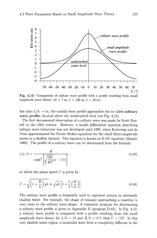
Fig. 4.12: Comparison of solitary wave profile with a profile resulting from small
amplitude wave theory (H = 7 m, L = 150 m, h = 10 m)
the ratio L / h ~ 00, the cnoidal wave profile approaches the so called solitary
wave profile, located above the undisturbed level (see Fig. 4.12).
The first documented observation of a solitary wave was made by Scott Russell in the 19th century. However, a model differential equation describing
solitary wave behaviour was not developed until 1895, when Korteweg and de
Vries approximated the Navier Stokes equations for the small finite-amplitude
waves in a shallow channel. This equation is known as K-dV equation (Massel,
1989). The profile of a solitary wave can be determined from the formula:
((x,t) =
[
] '
cosh 2 V!~(x -Gt)
H
( 4.43)
in which the phase speed G is given by:
G = J (1 + ~) gh ~ # [1 + ~ (~) ] .
( 4.44)
The solitary wave profile is frequently used to represent motion in extremely
shallow water. For example, the shape of tsunami approaching a coastline is
very close to the solitary wave shape. A computer program for determining
a solitary wave profile is given in Appendix D (program D.42). In Fig. 4.12,
a solitary wave profile is compared with a profile resulting from the small
amplitude wave theory for L/h = 15 and H /h = 0.7; thus U = 157. In this
very shallow water region, a sinusoidal wave form is completely different to the
S:8
~7
.~ 6
~
:> 5
~
~ 4
3
2
1
solitary wave profile
small amplitude
wave profile
123
o ~==~~--~~~~~~--------~r-~~===--1
-2
-3
-4 ~'-"-r'-,,-r.-,,'-,,'+'-,,-''-,,-''-,,-r'-,,
-70 -60 -50 -40 -30 -20 -10 0 10 20 30 40 50 60 70
L/2
Fig. 4.12: Comparison of solitary wave profile with a profile resulting from small
amplitude wave theory (H = 7 m, L = 150 m, h = 10 m)
the ratio L / h ~ 00, the cnoidal wave profile approaches the so called solitary
wave profile, located above the undisturbed level (see Fig. 4.12).
The first documented observation of a solitary wave was made by Scott Russell in the 19th century. However, a model differential equation describing
solitary wave behaviour was not developed until 1895, when Korteweg and de
Vries approximated the Navier Stokes equations for the small finite-amplitude
waves in a shallow channel. This equation is known as K-dV equation (Massel,
1989). The profile of a solitary wave can be determined from the formula:
((x,t) =
[
] '
cosh 2 V!~(x -Gt)
H
( 4.43)
in which the phase speed G is given by:
G = J (1 + ~) gh ~ # [1 + ~ (~) ] .
( 4.44)
The solitary wave profile is frequently used to represent motion in extremely
shallow water. For example, the shape of tsunami approaching a coastline is
very close to the solitary wave shape. A computer program for determining
a solitary wave profile is given in Appendix D (program D.42). In Fig. 4.12,
a solitary wave profile is compared with a profile resulting from the small
amplitude wave theory for L/h = 15 and H /h = 0.7; thus U = 157. In this
very shallow water region, a sinusoidal wave form is completely different to the