

70
2. Basic Finite-Difference Methods
1.5
lAI
1.0
0.5
C - - --------------, ' . .
1.0
0.75
0.5
0.25
'
o
0.0
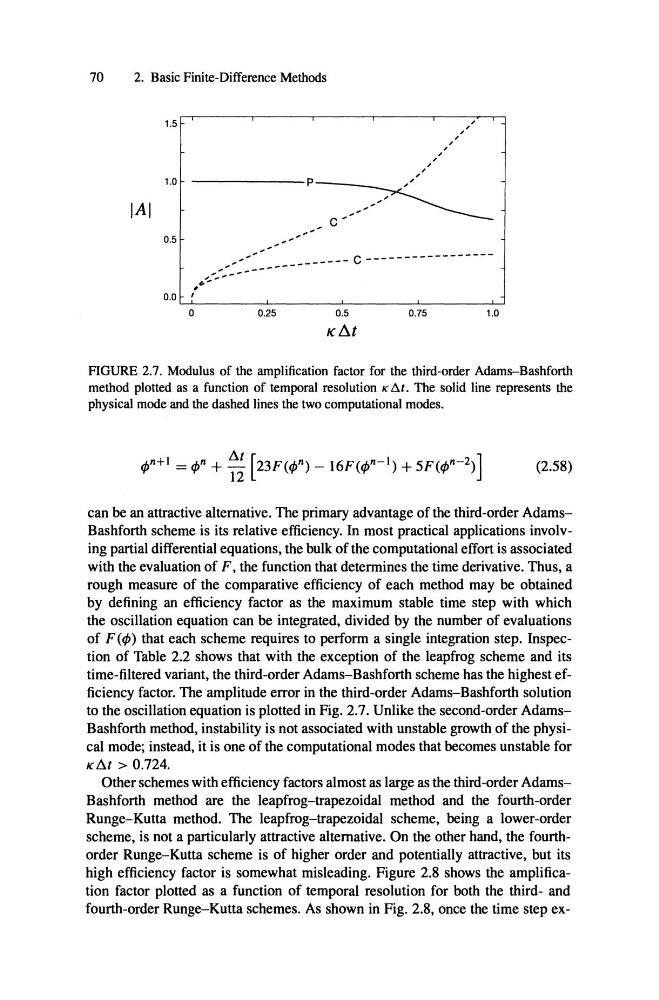
FIGURE 2.7. Modulus of the amplification factor for the third-order Adams-Bashforth
method plotted as a function of temporal resolution K flt . The solid line represents the
physical mode and the dashed lines the two computational modes .
(2.58)
can be an attractive alternative. The primary advantage of the third-order AdamsBashforth scheme is its relative efficiency. In most practical applications involving partial differential equations, the bulk of the computational effort is associated
with the evaluation of F , the function that determines the time derivative. Thus, a
rough measure of the comparative efficiency of each method may be obtained
by defining an efficiency factor as the maximum stable time step with which
the oscillation equation can be integrated, divided by the number of evaluations
of F( time-filtered variant, the third-order Adams-Bashforth scheme has the highest efficiency factor. The amplitude error in the third-order Adams-Bashforth solution
to the oscillation equation is plotted in Fig. 2.7. Unlike the second-order AdamsBashforth method, instability is not associated with unstable growth of the physical mode; instead, it is one of the computational modes that becomes unstable for
KM> 0.724.
Other schemes with efficiency factors almost as large as the third-order AdamsBashforth method are the leapfrog-trapezoidal method and the fourth-order
Runge-Kutta method . The leapfrog-trapezoidal scheme, being a lower-order
scheme, is not a particularly attractive alternative. On the other hand, the fourthorder Runge-Kutta scheme is of higher order and potentially attractive, but its
high efficiency factor is somewhat misleading. Figure 2.8 shows the amplification factor plotted as a function of temporal resolution for both the third- and
fourth-order Runge-Kutta schemes. As shown in Fig. 2.8, once the time step ex-
2. Basic Finite-Difference Methods
1.5
lAI
1.0
0.5
C - - --------------, ' . .
1.0
0.75
0.5
0.25
'
o
0.0
FIGURE 2.7. Modulus of the amplification factor for the third-order Adams-Bashforth
method plotted as a function of temporal resolution K flt . The solid line represents the
physical mode and the dashed lines the two computational modes .
(2.58)
can be an attractive alternative. The primary advantage of the third-order AdamsBashforth scheme is its relative efficiency. In most practical applications involving partial differential equations, the bulk of the computational effort is associated
with the evaluation of F , the function that determines the time derivative. Thus, a
rough measure of the comparative efficiency of each method may be obtained
by defining an efficiency factor as the maximum stable time step with which
the oscillation equation can be integrated, divided by the number of evaluations
of F( time-filtered variant, the third-order Adams-Bashforth scheme has the highest efficiency factor. The amplitude error in the third-order Adams-Bashforth solution
to the oscillation equation is plotted in Fig. 2.7. Unlike the second-order AdamsBashforth method, instability is not associated with unstable growth of the physical mode; instead, it is one of the computational modes that becomes unstable for
KM> 0.724.
Other schemes with efficiency factors almost as large as the third-order AdamsBashforth method are the leapfrog-trapezoidal method and the fourth-order
Runge-Kutta method . The leapfrog-trapezoidal scheme, being a lower-order
scheme, is not a particularly attractive alternative. On the other hand, the fourthorder Runge-Kutta scheme is of higher order and potentially attractive, but its
high efficiency factor is somewhat misleading. Figure 2.8 shows the amplification factor plotted as a function of temporal resolution for both the third- and
fourth-order Runge-Kutta schemes. As shown in Fig. 2.8, once the time step ex-