

66
2. Basic Finite-Difference Methods
1.5
p
1.0 - - - - - - - _ . /
lAI
0.5
... -- --... - ... --C...
-----0.0
--- --_ .... -
_
o
0,4
0.8
1.2
«S:
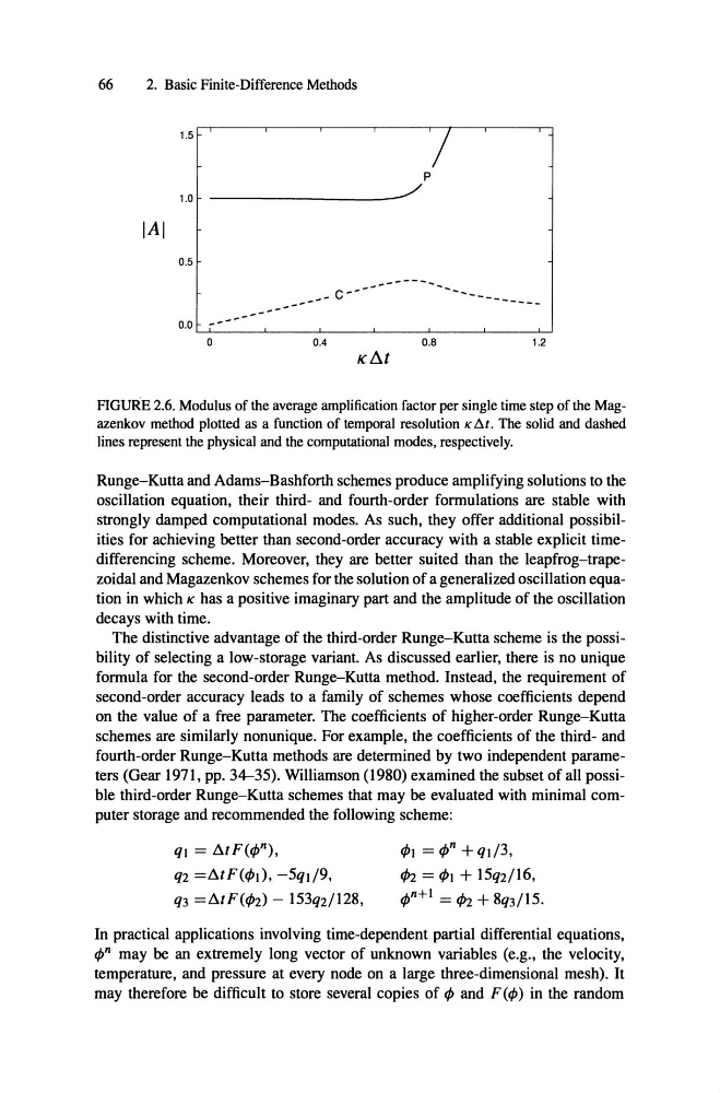
FIGURE 2.6. Modulus of the average amplification factor per single time step of the Magazenkov method plotted as a function of temporal resolution K 6.1. The solid and dashed
lines represent the physical and the computationaI modes , respectively.
Runge-Kutta and Adams-Bashforth schemes produce ampIifying solutions to the
oscillation equation, their third- and fourth-order formulations are stable with
strongly damped computational modes. As such, they offer additional possibilities for achieving better than second-order accuracy with a stable explicit timedifferencing scheme. Moreover, they are better suited than the leapfrog-trapezoidal and Magazenkov schemes for the solution of a generalized oscillation equation in which K has a positive imaginary part and the amplitude of the oscillation
decays with time.
The distinctive advantage of the third-order Runge-Kutta scheme is the possibility of selecting a low-storage variant. As discussed earlier, there is no unique
formula for the second-order Runge-Kutta method . Instead , the requirement of
second-order accuracy leads to a family of schemes whose coefficients depend
on the value of a free parameter. The coefficients of higher-order Runge-Kutta
schemes are similarly nonunique. For example, the coefficients of the third- and
fourth-order Runge-Kutta methods are determined by two independent parameters (Gear 1971, pp. 34-35). Williamson (1980) examined the subset of all possible third-order Runge-Kutta schemes that may be evaluated with minimal computer storage and recommended the following scheme:
qt = !ltF(cP n ) ,
qz =!ltF(cPt) , -5qJ!9,
q3 =!ltF(cP2) - 153q2/128,
cPt = cP
n
+ qt 13,
cP2 = cPt + 15q2/16,
cP
n
+
t = cP2 + 8q3/15.
In practical applications involving time-dependent partial differential equations,
cP n may be an extremely long vector of unknown variables (e.g., the velocity,
temperature, and pressure at every node on a large three-dimensional mesh). It
may therefore be difficult to store several copies of cP and F(cP) in the random
2. Basic Finite-Difference Methods
1.5
p
1.0 - - - - - - - _ . /
lAI
0.5
... -- --... - ... --C...
-----0.0
--- --_ .... -
_
o
0,4
0.8
1.2
«S:
FIGURE 2.6. Modulus of the average amplification factor per single time step of the Magazenkov method plotted as a function of temporal resolution K 6.1. The solid and dashed
lines represent the physical and the computationaI modes , respectively.
Runge-Kutta and Adams-Bashforth schemes produce ampIifying solutions to the
oscillation equation, their third- and fourth-order formulations are stable with
strongly damped computational modes. As such, they offer additional possibilities for achieving better than second-order accuracy with a stable explicit timedifferencing scheme. Moreover, they are better suited than the leapfrog-trapezoidal and Magazenkov schemes for the solution of a generalized oscillation equation in which K has a positive imaginary part and the amplitude of the oscillation
decays with time.
The distinctive advantage of the third-order Runge-Kutta scheme is the possibility of selecting a low-storage variant. As discussed earlier, there is no unique
formula for the second-order Runge-Kutta method . Instead , the requirement of
second-order accuracy leads to a family of schemes whose coefficients depend
on the value of a free parameter. The coefficients of higher-order Runge-Kutta
schemes are similarly nonunique. For example, the coefficients of the third- and
fourth-order Runge-Kutta methods are determined by two independent parameters (Gear 1971, pp. 34-35). Williamson (1980) examined the subset of all possible third-order Runge-Kutta schemes that may be evaluated with minimal computer storage and recommended the following scheme:
qt = !ltF(cP n ) ,
qz =!ltF(cPt) , -5qJ!9,
q3 =!ltF(cP2) - 153q2/128,
cPt = cP
n
+ qt 13,
cP2 = cPt + 15q2/16,
cP
n
+
t = cP2 + 8q3/15.
In practical applications involving time-dependent partial differential equations,
cP n may be an extremely long vector of unknown variables (e.g., the velocity,
temperature, and pressure at every node on a large three-dimensional mesh). It
may therefore be difficult to store several copies of cP and F(cP) in the random