

1.3Strategies for Numerical Approximation
31
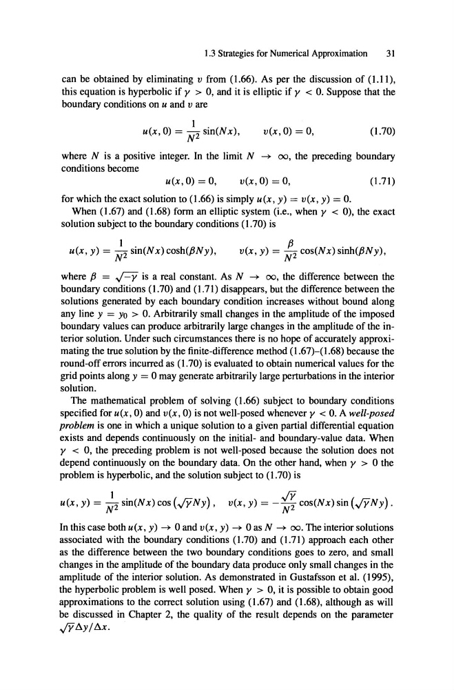
can be obtained by eliminating v from (1.66). As per the discussion of (l.ll),
this equation is hyperbolic if y > 0, and it is elliptic if y < O. Suppose that the
boundary conditions on u and v are
1 .
u(x,O) = N2 sm(Nx),
(1.70)
v(x, 0) = 0,
where N is a positive integer. In the limit N
00, the preceding boundary
conditions become
U(x,O) = 0,
(1.71)
v(x,O) = 0,
for which the exact solution to (1.66) is simply u(x, y) = v(x, y) = O.
When (1.67) and (1.68) form an elliptic system (i.e., when y < 0), the exact
solution subject to the boundary conditions (1.70) is
v(x, y) = :2cos( Nx) sinh(ßNy) ,
u(x, y) =
1 .
N2 sm(Nx) cosh(ßNy),
where ß = .;-:::y is areal constant. As N 00, the difference between the
boundary conditions (1.70) and (1.71) disappears, but the difference between the
solutions generated by each boundary condition increases without bound along
any line y = Yo > O. Arbitrarily small changes in the amplitude of the imposed
boundary values can produce arbitrarily large changes in the amplitude of the interior solution. Under such circumstances there is no hope of accurate1y approximating the true solution by the finite-difference method (1.67)-(1.68) because the
round-off errors incurred as (1.70) is evaluated to obtain numerical values for the
grid points along y = 0 may generate arbitrarily large perturbations in the interior
solution.
The mathematical problem of solving (1.66) subject to boundary conditions
specified for u(x, 0) and v(x, 0) is not well-posed whenever y < O. A well-posed
problem is one in which a unique solution to a given partial differential equation
exists and depends continuously on the initial- and boundary-value data. When
y < 0, the preceding problem is not well-posed because the solution does not
depend continuously on the boundary data. On the othcr hand, when y > 0 the
problem is hyperbolic, and the solution subject to (1.70) is
u(x, y) =
sin(Nx) cos (.JYNY) , v(x, y) = - .;;: cos(Nx) sin (.JYNy).
In this case both u(x, y)
0 and v(x, y)
0 as N
00. The interior solutions
associated with the boundary conditions (1.70) and (1.71) approach each other
as the difference between the two boundary conditions goes to zero, and small
changes in the amplitude of the boundary data producc only small changes in the
amplitude of the interior solution . As demonstrated in Gustafsson et al. (1995),
the hyperbolic problem is weIl posed. When y > 0, it is possible to obtain good
approximations to the correct solution using (1.67) and (1.68), although as will
be discussed in Chapter 2, the quality of the result depends on the parameter
.JYf:1yjtu.
31
can be obtained by eliminating v from (1.66). As per the discussion of (l.ll),
this equation is hyperbolic if y > 0, and it is elliptic if y < O. Suppose that the
boundary conditions on u and v are
1 .
u(x,O) = N2 sm(Nx),
(1.70)
v(x, 0) = 0,
where N is a positive integer. In the limit N
00, the preceding boundary
conditions become
U(x,O) = 0,
(1.71)
v(x,O) = 0,
for which the exact solution to (1.66) is simply u(x, y) = v(x, y) = O.
When (1.67) and (1.68) form an elliptic system (i.e., when y < 0), the exact
solution subject to the boundary conditions (1.70) is
v(x, y) = :2cos( Nx) sinh(ßNy) ,
u(x, y) =
1 .
N2 sm(Nx) cosh(ßNy),
where ß = .;-:::y is areal constant. As N 00, the difference between the
boundary conditions (1.70) and (1.71) disappears, but the difference between the
solutions generated by each boundary condition increases without bound along
any line y = Yo > O. Arbitrarily small changes in the amplitude of the imposed
boundary values can produce arbitrarily large changes in the amplitude of the interior solution. Under such circumstances there is no hope of accurate1y approximating the true solution by the finite-difference method (1.67)-(1.68) because the
round-off errors incurred as (1.70) is evaluated to obtain numerical values for the
grid points along y = 0 may generate arbitrarily large perturbations in the interior
solution.
The mathematical problem of solving (1.66) subject to boundary conditions
specified for u(x, 0) and v(x, 0) is not well-posed whenever y < O. A well-posed
problem is one in which a unique solution to a given partial differential equation
exists and depends continuously on the initial- and boundary-value data. When
y < 0, the preceding problem is not well-posed because the solution does not
depend continuously on the boundary data. On the othcr hand, when y > 0 the
problem is hyperbolic, and the solution subject to (1.70) is
u(x, y) =
sin(Nx) cos (.JYNY) , v(x, y) = - .;;: cos(Nx) sin (.JYNy).
In this case both u(x, y)
0 and v(x, y)
0 as N
00. The interior solutions
associated with the boundary conditions (1.70) and (1.71) approach each other
as the difference between the two boundary conditions goes to zero, and small
changes in the amplitude of the boundary data producc only small changes in the
amplitude of the interior solution . As demonstrated in Gustafsson et al. (1995),
the hyperbolic problem is weIl posed. When y > 0, it is possible to obtain good
approximations to the correct solution using (1.67) and (1.68), although as will
be discussed in Chapter 2, the quality of the result depends on the parameter
.JYf:1yjtu.