

30
I. Introduction
soJ
-.'
S2 J
_
I
2.
x
J
tly
v,!+1 - v'!
J
tly
-
2tlx
(1.67)
(1.68)
I
o
- J + J+I
-:!-'---"';:""":" = 0,
v'! - v'!
JI
2tlx
J + Y --:"'---"';:""- J+I J-I = 0,
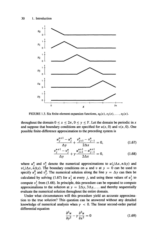
FIGURE 1.3. Six finite-element expansion functions, so(x), SI (x), . .. , ss(x) .
throughout the domain 0 :s x :s 21T, 0 :s y :s Y. Let the domain be periodic in x
and suppose that boundary conditions are specified for u(x , 0) and v(x , 0) . One
possible finite-difference approximation to the preceding system is
where u'J and vj denote the numerical approximations to ui j S», ntly) and
v(jtlx, ntly) . The boundary conditions on u and v at y = 0 can be used to
specify
and
The numerical solution along the line y = tly can then be
calculated by solving (1.67) for u} at every i, and using these values of u} to
compute v} from (1.68). In principle, this procedure can be repeated to compute
approximations to the solution at y = 2tly, 3tly , .. . and thereby sequentially
evaluate the numerical solution throughout the entire domain.
Under what circumstances will this procedure yield an accurate approximation to the true solution? This question can be answered without any detailed
knowledge of numerical analysis when y < O. The linear second-order partial
differential equation
(1.69)
I. Introduction
soJ
-.'
S2 J
_
I
2.
x
J
tly
v,!+1 - v'!
J
tly
-
2tlx
(1.67)
(1.68)
I
o
- J + J+I
-:!-'---"';:""":" = 0,
v'! - v'!
JI
2tlx
J + Y --:"'---"';:""- J+I J-I = 0,
FIGURE 1.3. Six finite-element expansion functions, so(x), SI (x), . .. , ss(x) .
throughout the domain 0 :s x :s 21T, 0 :s y :s Y. Let the domain be periodic in x
and suppose that boundary conditions are specified for u(x , 0) and v(x , 0) . One
possible finite-difference approximation to the preceding system is
where u'J and vj denote the numerical approximations to ui j S», ntly) and
v(jtlx, ntly) . The boundary conditions on u and v at y = 0 can be used to
specify
and
The numerical solution along the line y = tly can then be
calculated by solving (1.67) for u} at every i, and using these values of u} to
compute v} from (1.68). In principle, this procedure can be repeated to compute
approximations to the solution at y = 2tly, 3tly , .. . and thereby sequentially
evaluate the numerical solution throughout the entire domain.
Under what circumstances will this procedure yield an accurate approximation to the true solution? This question can be answered without any detailed
knowledge of numerical analysis when y < O. The linear second-order partial
differential equation
(1.69)