

8.3 Two-Dimensional Stratified Flow
421
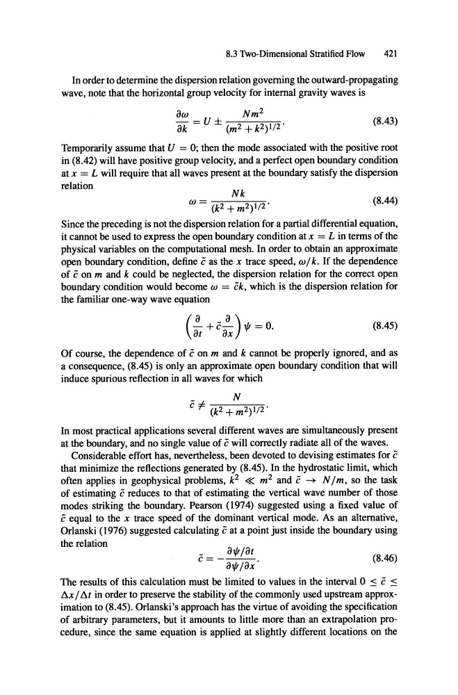
In order to determine the dispersion relation governing the outward-propagating
wave, note that the horizontal group velocity for internal gravity waves is
aw
Nm
2
ak = U ± (m2 + k2)1/2·
(8.43)
Temporarily assume that U = 0; then the mode associated with the positive root
in (8.42) will have positive group velocity, and a perfect open boundary condition
at x = L will require that an waves present at the boundary satisfy the dispersion
relation
Nk
w = (k 2 + m 2 )1/2 .
(8.44)
Since the preceding is not the dispersion relation for a partial differential equation,
it cannot be used to express the open boundary condition at x = L in terms of the
physical variables on the computational mesh. In order to obtain an approximate
open boundary condition, define cas the x trace speed, ta]k. If the dependence
of con m and k could be neglected, the dispersion relation for the correct open
boundary condition would become w = Ck, which is the dispersion relation for
the familiar one -way wave equation
( - a +c- _a ) 1{! =
(8.45)
Of course, the dependence of con m and k cannot be properly ignored, and as
a consequence, (8.45) is only an approximate open boundary condition that will
induce spurious reftection in an waves for which
In most practical applications several different waves are simultaneously present
at the boundary, and no single value of cwill correctly radiate an of the waves.
Considerable effort has, nevertheless, been devoted to devising estimates for c
that minimize the reftections generated by (8.45). In the hydrostatic limit, which
often applies in geophysical problems, k 2 « m 2 and c N Im, so the task
of estimating creduces to that of estimating the vertical wave number of those
modes striking the boundary. Pearson (1974) suggested using a fixed value of
cequal to the x trace speed of the dominant vertical mode . As an alternative,
Orlanski (1976) suggested calculating cat a point just inside the boundary using
the relation
(8.46)
The results of this calculation must be limited to values in the interval 0 :5 c :5
tu I!i.t in order to preserve the stability of the commonly used upstream approximation to (8.45) . Orlanski's approach has the virtue of avoiding the specification
of arbitrary parameters, but it amounts to little more than an extrapolation procedure, since the same equation is applied at slightly different locations on the
421
In order to determine the dispersion relation governing the outward-propagating
wave, note that the horizontal group velocity for internal gravity waves is
aw
Nm
2
ak = U ± (m2 + k2)1/2·
(8.43)
Temporarily assume that U = 0; then the mode associated with the positive root
in (8.42) will have positive group velocity, and a perfect open boundary condition
at x = L will require that an waves present at the boundary satisfy the dispersion
relation
Nk
w = (k 2 + m 2 )1/2 .
(8.44)
Since the preceding is not the dispersion relation for a partial differential equation,
it cannot be used to express the open boundary condition at x = L in terms of the
physical variables on the computational mesh. In order to obtain an approximate
open boundary condition, define cas the x trace speed, ta]k. If the dependence
of con m and k could be neglected, the dispersion relation for the correct open
boundary condition would become w = Ck, which is the dispersion relation for
the familiar one -way wave equation
( - a +c- _a ) 1{! =
(8.45)
Of course, the dependence of con m and k cannot be properly ignored, and as
a consequence, (8.45) is only an approximate open boundary condition that will
induce spurious reftection in an waves for which
In most practical applications several different waves are simultaneously present
at the boundary, and no single value of cwill correctly radiate an of the waves.
Considerable effort has, nevertheless, been devoted to devising estimates for c
that minimize the reftections generated by (8.45). In the hydrostatic limit, which
often applies in geophysical problems, k 2 « m 2 and c N Im, so the task
of estimating creduces to that of estimating the vertical wave number of those
modes striking the boundary. Pearson (1974) suggested using a fixed value of
cequal to the x trace speed of the dominant vertical mode . As an alternative,
Orlanski (1976) suggested calculating cat a point just inside the boundary using
the relation
(8.46)
The results of this calculation must be limited to values in the interval 0 :5 c :5
tu I!i.t in order to preserve the stability of the commonly used upstream approximation to (8.45) . Orlanski's approach has the virtue of avoiding the specification
of arbitrary parameters, but it amounts to little more than an extrapolation procedure, since the same equation is applied at slightly different locations on the