

28
I. Introduction
(a)
f
o
x
2"
f
o
x
2"
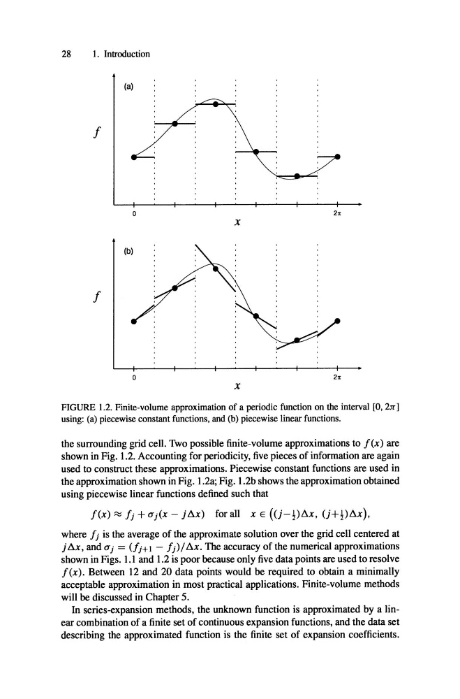
FIGURE 1.2. Finite-volume approximation of a periodic function on the interval [0, 2JT]
using: (a) piecewise constant functions, and (b) piecewise linear functions.
the surrounding grid cell. Two possible finite-volume approximations to f(x) are
shown in Fig. 1.2. Accounting for periodicity, five pieces of information are again
used to construct these approximations. Piecewise constant functions are used in
the approximation shown in Fig. I.2a; Fig. I.2b shows the approximation obtained
using piecewise linear functions defined such that
f(x)
/i +aj(x - jt:u) forall x E
where fj is the average of the approximate solution over the grid cell centered at
j ßX, and aj = (fJ+ 1 - /i) / S». The accuracy of the numerical approximations
shown in Figs. 1.1 and 1.2 is poor because only five data points are used to resolve
f(x). Between 12 and 20 data points would be required to obtain a minimally
acceptable approximation in most practical applications. Finite-volume methods
will be discussed in Chapter 5.
In series-expansion methods, the unknown function is approximated by a linear combination of a finite set of continuous expansion functions, and the data set
describing the approximated function is the finite set of expansion coefficients.
I. Introduction
(a)
f
o
x
2"
f
o
x
2"
FIGURE 1.2. Finite-volume approximation of a periodic function on the interval [0, 2JT]
using: (a) piecewise constant functions, and (b) piecewise linear functions.
the surrounding grid cell. Two possible finite-volume approximations to f(x) are
shown in Fig. 1.2. Accounting for periodicity, five pieces of information are again
used to construct these approximations. Piecewise constant functions are used in
the approximation shown in Fig. I.2a; Fig. I.2b shows the approximation obtained
using piecewise linear functions defined such that
f(x)
/i +aj(x - jt:u) forall x E
where fj is the average of the approximate solution over the grid cell centered at
j ßX, and aj = (fJ+ 1 - /i) / S». The accuracy of the numerical approximations
shown in Figs. 1.1 and 1.2 is poor because only five data points are used to resolve
f(x). Between 12 and 20 data points would be required to obtain a minimally
acceptable approximation in most practical applications. Finite-volume methods
will be discussed in Chapter 5.
In series-expansion methods, the unknown function is approximated by a linear combination of a finite set of continuous expansion functions, and the data set
describing the approximated function is the finite set of expansion coefficients.