

1.3Strategies for Numerical Approximation
27
f
o
x
21l
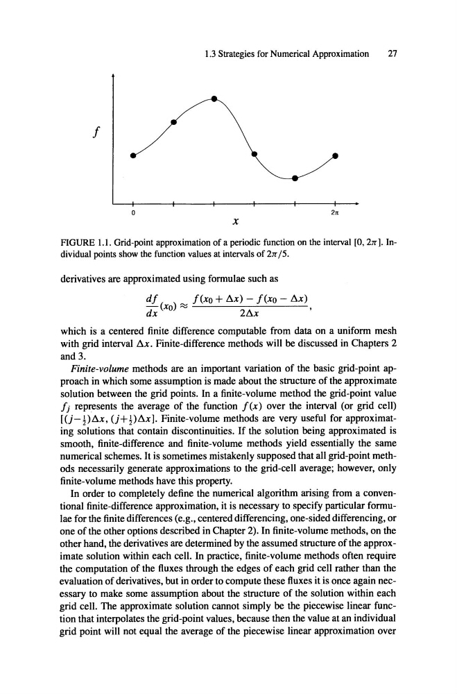
FIGURE 1.1.Grid-point approxirnation of a periodic function on the interval [0, 2][]. Individual points show the function values at intervals of 2][/5.
derivatives are approximated using formulae such as
df
dx (xo)
f(xo + ö-x) - f(xo - ö-x)
2ö-x
'
which is a centered finite difference computable from data on a uniform mesh
with grid interval Ö-x. Finite-difference methods will be discussed in Chapters 2
and 3.
Finite-volume methods are an important variation of the basic grid-point approach in which some assumption is made about the structure of the approximate
solution between the grid points. In a finite-volume method the grid-point value
fj represents the average of the function fex) over the interval (or grid cell)
((j- pö-x , (j+pö-x]. Finite-volume methods are very useful for approximating solutions that contain discontinuities. If the solution being approximated is
smooth, finite-difference and finite-volume methods yield essentially the same
numerical schemes. It is sometimes mistakenly supposed that all grid-point rnethods necessarily generate approximations to the grid-cell average; however, only
finite-volume methods have this property.
In order to completely define the numerical algorithm arising from a conventional finite-difference approximation, it is necessary to specify particular formulae for the finite differences (e.g., centered differencing, one-sided differencing, or
one of the other options described in Chapter 2). In finite-volume methods, on the
other hand, the derivatives are determined by the assumed structure of the approximate solution within each cell. In practice, finite-volume methods often require
the computation of the fluxes through the edges of each grid cell rather than the
evaluation of derivatives, but in order to compute these fluxes it is once again necessary to make some assumption about the structure of the solution within each
grid cell. The approximate solution cannot simply be the piecewise linear function that interpolates the grid-point values, because then the value at an individual
grid point will not equal the average of the piecewise linear approximation over
27
f
o
x
21l
FIGURE 1.1.Grid-point approxirnation of a periodic function on the interval [0, 2][]. Individual points show the function values at intervals of 2][/5.
derivatives are approximated using formulae such as
df
dx (xo)
f(xo + ö-x) - f(xo - ö-x)
2ö-x
'
which is a centered finite difference computable from data on a uniform mesh
with grid interval Ö-x. Finite-difference methods will be discussed in Chapters 2
and 3.
Finite-volume methods are an important variation of the basic grid-point approach in which some assumption is made about the structure of the approximate
solution between the grid points. In a finite-volume method the grid-point value
fj represents the average of the function fex) over the interval (or grid cell)
((j- pö-x , (j+pö-x]. Finite-volume methods are very useful for approximating solutions that contain discontinuities. If the solution being approximated is
smooth, finite-difference and finite-volume methods yield essentially the same
numerical schemes. It is sometimes mistakenly supposed that all grid-point rnethods necessarily generate approximations to the grid-cell average; however, only
finite-volume methods have this property.
In order to completely define the numerical algorithm arising from a conventional finite-difference approximation, it is necessary to specify particular formulae for the finite differences (e.g., centered differencing, one-sided differencing, or
one of the other options described in Chapter 2). In finite-volume methods, on the
other hand, the derivatives are determined by the assumed structure of the approximate solution within each cell. In practice, finite-volume methods often require
the computation of the fluxes through the edges of each grid cell rather than the
evaluation of derivatives, but in order to compute these fluxes it is once again necessary to make some assumption about the structure of the solution within each
grid cell. The approximate solution cannot simply be the piecewise linear function that interpolates the grid-point values, because then the value at an individual
grid point will not equal the average of the piecewise linear approximation over