

7.6 PrimitiveEquation Models
379
have been proposed that guarantee exact cancellation of the vertical pressure gradient between the last two terms in (7.102) whenever the vertical profiles of temperature and pressure have a specified functional relation , such as T = a In(p)+b
(Corby et al. 1972; Nakamura 1978; Simmons and Burridge 1981). Mesinger
(1984) suggested using "n -coordinates" in which the mountain slopes are discretized as vertical steps at the grid interfaces with flat terrain between each
step. More details and additional techniques for the treatment of pressure -gradient
errors over mountains in hydrostatic atmospheric models are presented in the review by Mesinger and Jani ö(1985).
7.6.2 Spectral Representation ofthe Horizontal Structure
Global primitive-equation models often use spherical harmonics to represent the
latitudinal and longitudinal variation of the forecast variables. In the following
sections we present the basic numerical procedures for creating a spectral approximation to the a-coordinate equations in a giobai atmospheric model. Tbe
approach is similar to that in Hoskins and Simmons (1975) and Bourke (1974),
which may be consulted for additional details. The latitudinal and longitudinal
variations in each field will be approximated using spherical harmonics, and the
vertical variations will be represented using grid-point methods.
As was the case for the global shallow-water model described in Section 4.4.4,
the spectral representation of the horizontal velocity field is facilitated by expressing the horizontal momentum equations in terms of the vertical vorticity I;
and the divergence 8. In order to integrate this system easily using semi-implicit
time-differencing , it is also helpful to divide the temperature into a horizontally
uniform reference state and a perturbation such that T = T(a) + T' . Using the
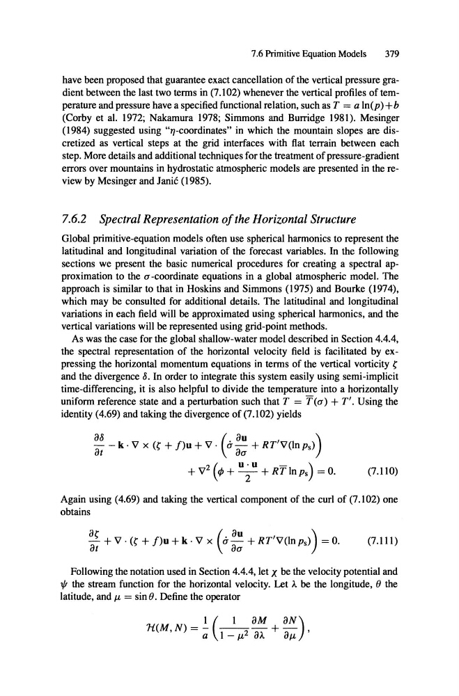
identity (4.69) and taking the divergence of (7.102) yields
- 88 - k . V x (I; + f)n + V · (. a - 8u + RT V(ln Ps)
I
)
81
2(
8a
+ V ,p + -2u v u + RT In Ps
-
) = O.
(7.110)
Again using (4.69) and taking the vertical component of the curl of (7.102) one
obtains
-+V ·(I;+f)n+k·Vx
81;
(. a-+RT'V(lnps) 8n
) =0.
(7.111)
81
8a
Following the notation used in Section 4.4.4, let X be the velocity potential and
1/1 the stream function for the horizontal velocity. Let A be tbe longitude, () the
latitude, and JL = sin (). Define the operator
I (
1 8M
8N)
1t(M, N) =
1 _ JL2 ai" + 8JL '
379
have been proposed that guarantee exact cancellation of the vertical pressure gradient between the last two terms in (7.102) whenever the vertical profiles of temperature and pressure have a specified functional relation , such as T = a In(p)+b
(Corby et al. 1972; Nakamura 1978; Simmons and Burridge 1981). Mesinger
(1984) suggested using "n -coordinates" in which the mountain slopes are discretized as vertical steps at the grid interfaces with flat terrain between each
step. More details and additional techniques for the treatment of pressure -gradient
errors over mountains in hydrostatic atmospheric models are presented in the review by Mesinger and Jani ö(1985).
7.6.2 Spectral Representation ofthe Horizontal Structure
Global primitive-equation models often use spherical harmonics to represent the
latitudinal and longitudinal variation of the forecast variables. In the following
sections we present the basic numerical procedures for creating a spectral approximation to the a-coordinate equations in a giobai atmospheric model. Tbe
approach is similar to that in Hoskins and Simmons (1975) and Bourke (1974),
which may be consulted for additional details. The latitudinal and longitudinal
variations in each field will be approximated using spherical harmonics, and the
vertical variations will be represented using grid-point methods.
As was the case for the global shallow-water model described in Section 4.4.4,
the spectral representation of the horizontal velocity field is facilitated by expressing the horizontal momentum equations in terms of the vertical vorticity I;
and the divergence 8. In order to integrate this system easily using semi-implicit
time-differencing , it is also helpful to divide the temperature into a horizontally
uniform reference state and a perturbation such that T = T(a) + T' . Using the
identity (4.69) and taking the divergence of (7.102) yields
- 88 - k . V x (I; + f)n + V · (. a - 8u + RT V(ln Ps)
I
)
81
2(
8a
+ V ,p + -2u v u + RT In Ps
-
) = O.
(7.110)
Again using (4.69) and taking the vertical component of the curl of (7.102) one
obtains
-+V ·(I;+f)n+k·Vx
81;
(. a-+RT'V(lnps) 8n
) =0.
(7.111)
81
8a
Following the notation used in Section 4.4.4, let X be the velocity potential and
1/1 the stream function for the horizontal velocity. Let A be tbe longitude, () the
latitude, and JL = sin (). Define the operator
I (
1 8M
8N)
1t(M, N) =
1 _ JL2 ai" + 8JL '