

7.1 The ProjectionMethod
339
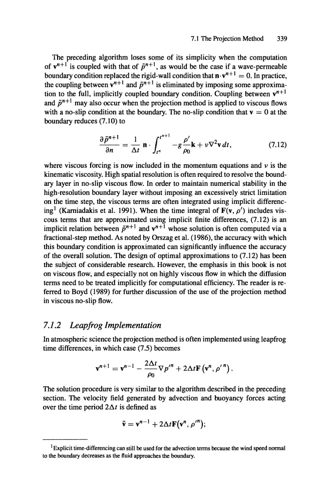
The preceding algorithm loses some of its simplicity when the computation
of yn+1 is coupled with that of jjn+ 1 , as would be the case if a wave-permeable
boundary condition replaced the rigid-wall condition that ß·yn+l = O. In practice ,
the coupling between yn+ 1 and jjn+ 1 is eliminated by imposing some approximation to the full, implicitly coupled boundary condition. Coupling between yn+I
and jjn+ 1 mayaiso occur when the projection method is applied to viscous flows
with a no-slip condition at the boundary. The no-slip condition that v = 0 at the
1
-g-k+vV v dt ,
2
Po
boundary reduces (7.10) to
a -n+l
P
1
1/
n +
P
I
- - = -
an
D.t
/n
ß ·
(7.12)
where viscous forcing is now included in the momentum equations and v is the
kinematic viscosity. High spatial resolution is often required to resolve the boundary layer in no-slip viscous flow. In order to maintain numerical stability in the
high-resolution boundary layer without imposing an excessively strict limitation
on the time step, the viscous terms are often integrated using implicit differencing ' (Karniadakis et aI. 1991). When the time integral of Ftv, p') includes viscous terms that are approximated using implicit finite differences, (7.12) is an
implicit relation between r: 1 and yn+ 1 whose solution is often computed via a
fractional -step method. As noted by Orszag et aI. (1986), the accuracy with which
this boundary condition is approximated can significantly influence the accuracy
of the overall solution . The design of optimal approximations to (7.12) has been
the subject of considerable research. However, the emphasis in this book is not
on viscous flow, and especially not on highly viscous flow in which the diffusion
terms need to be treated implicitly for computational efficiency. The reader is referred to Boyd (1989) for further discussion of the use of the projection method
in viscous no-slip flow.
7.1.2 Leapfrog Implementation
In atmospheric science the projection method is often implemented using leapfrog
time differences, in which case (7.5) becomes
The solution procedure is very similar to the algorithm described in the preceding
section. The velocity field generated by advection and buoyancy forces acting
over the time period 2D.t is defined as
I Explicittime-differencing can still be used for the advectionterms becausethe wind speed normal
to the boundarydecreases as the fluidapproachesthe boundary.
339
The preceding algorithm loses some of its simplicity when the computation
of yn+1 is coupled with that of jjn+ 1 , as would be the case if a wave-permeable
boundary condition replaced the rigid-wall condition that ß·yn+l = O. In practice ,
the coupling between yn+ 1 and jjn+ 1 is eliminated by imposing some approximation to the full, implicitly coupled boundary condition. Coupling between yn+I
and jjn+ 1 mayaiso occur when the projection method is applied to viscous flows
with a no-slip condition at the boundary. The no-slip condition that v = 0 at the
1
-g-k+vV v dt ,
2
Po
boundary reduces (7.10) to
a -n+l
P
1
1/
n +
P
I
- - = -
an
D.t
/n
ß ·
(7.12)
where viscous forcing is now included in the momentum equations and v is the
kinematic viscosity. High spatial resolution is often required to resolve the boundary layer in no-slip viscous flow. In order to maintain numerical stability in the
high-resolution boundary layer without imposing an excessively strict limitation
on the time step, the viscous terms are often integrated using implicit differencing ' (Karniadakis et aI. 1991). When the time integral of Ftv, p') includes viscous terms that are approximated using implicit finite differences, (7.12) is an
implicit relation between r: 1 and yn+ 1 whose solution is often computed via a
fractional -step method. As noted by Orszag et aI. (1986), the accuracy with which
this boundary condition is approximated can significantly influence the accuracy
of the overall solution . The design of optimal approximations to (7.12) has been
the subject of considerable research. However, the emphasis in this book is not
on viscous flow, and especially not on highly viscous flow in which the diffusion
terms need to be treated implicitly for computational efficiency. The reader is referred to Boyd (1989) for further discussion of the use of the projection method
in viscous no-slip flow.
7.1.2 Leapfrog Implementation
In atmospheric science the projection method is often implemented using leapfrog
time differences, in which case (7.5) becomes
The solution procedure is very similar to the algorithm described in the preceding
section. The velocity field generated by advection and buoyancy forces acting
over the time period 2D.t is defined as
I Explicittime-differencing can still be used for the advectionterms becausethe wind speed normal
to the boundarydecreases as the fluidapproachesthe boundary.