

6.4 Alternative Trajectories
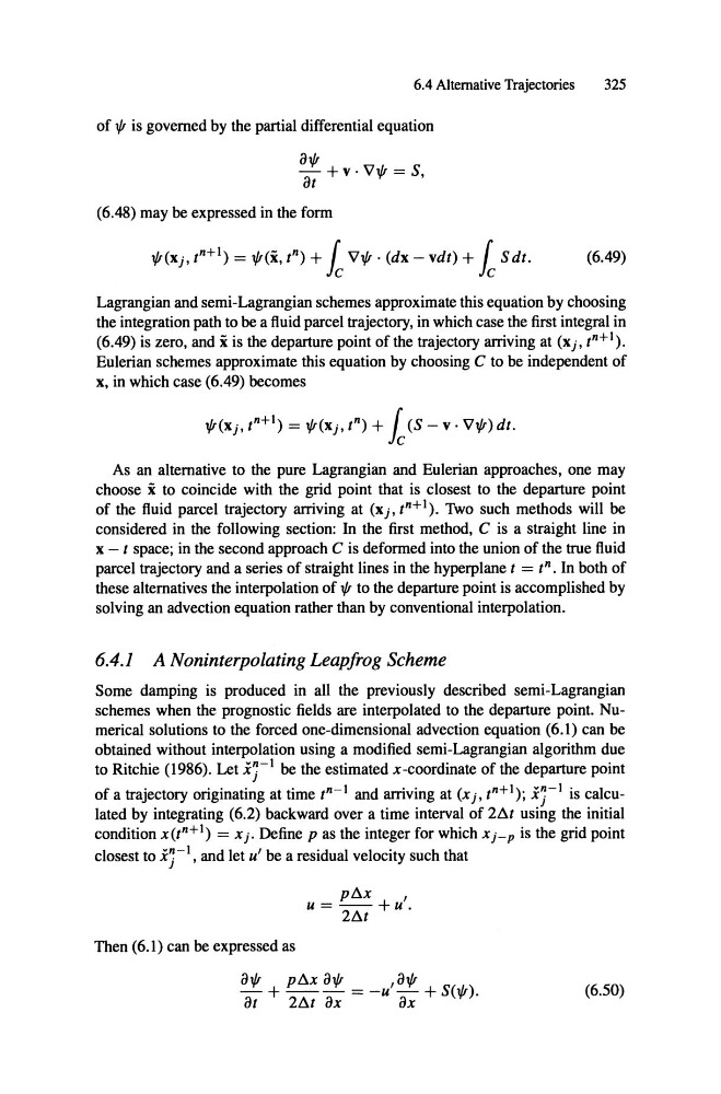
of 1/1 is governed by the partial differential equation
-
01/1
ot
+v · ' 111/1 = S '
325
(6.48) may be expressed in the form
(6.49)
Lagrangian and semi-Lagrangian schemes approximate this equation by choosing
the integration path to be a fluid parcel trajectory, in which case the first integral in
(6.49) is zero, and xis the departure point of the trajectory arriving at (xj , t n +
I ) .
Eulerian schemes approximate this equation by choosing C to be independent of
x, in which case (6.49) becomes
As an alternative to the pure Lagrangian and Eulerian approaches, one may
choose xto coincide with the grid point that is closest to the departure point
of the fluid parcel trajectory arriving at (X j, t n + I ) . Two such methods will be
considered in the following section: In the first method, C is a straight line in
x - t space ; in the second approach C is deformed into the union of the true fluid
parcel trajectory and aseries of straight lines in the hyperplane t = t", In both of
these alternatives the interpolation of 1/1 to the departure point is accomplished by
solving an advection equation rather than by conventional interpolation.
6.4.1 A Noninterpolating Leapjrog Scheme
Some damping is produced in all the previously described semi -Lagrangian
schemes when the prognostic fields are interpolated to the departure point. Numerical solutions to the forced one-dimensional advection equation (6.1) can be
obtained without interpolation using a modified serni-Lagrangian algorithm due
to Ritchie (1986). Let Ir
l be the estimated x-coordinate of the departure point
of a trajectory originating at time t n -
I and arriving at (x] , t n +
I ) ; Ir
l is calculated by integrating (6.2) backward over a time interval of 2!:J.t using the initial
condition x(t n + l ) = Xj . Define p as the integer for which Xj_p is the grid point
closest to IrI, and let u' be a residual velocity such that
p!:J.X
,
u=--+u.
2!:J.t
Then (6.1) can be expressed as
-
01/1
+
pSx 01/1
- - = -u
,01/1
- + S(1/I) .
ot
2!:J.t OX
OX
(6.50)
of 1/1 is governed by the partial differential equation
-
01/1
ot
+v · ' 111/1 = S '
325
(6.48) may be expressed in the form
(6.49)
Lagrangian and semi-Lagrangian schemes approximate this equation by choosing
the integration path to be a fluid parcel trajectory, in which case the first integral in
(6.49) is zero, and xis the departure point of the trajectory arriving at (xj , t n +
I ) .
Eulerian schemes approximate this equation by choosing C to be independent of
x, in which case (6.49) becomes
As an alternative to the pure Lagrangian and Eulerian approaches, one may
choose xto coincide with the grid point that is closest to the departure point
of the fluid parcel trajectory arriving at (X j, t n + I ) . Two such methods will be
considered in the following section: In the first method, C is a straight line in
x - t space ; in the second approach C is deformed into the union of the true fluid
parcel trajectory and aseries of straight lines in the hyperplane t = t", In both of
these alternatives the interpolation of 1/1 to the departure point is accomplished by
solving an advection equation rather than by conventional interpolation.
6.4.1 A Noninterpolating Leapjrog Scheme
Some damping is produced in all the previously described semi -Lagrangian
schemes when the prognostic fields are interpolated to the departure point. Numerical solutions to the forced one-dimensional advection equation (6.1) can be
obtained without interpolation using a modified serni-Lagrangian algorithm due
to Ritchie (1986). Let Ir
l be the estimated x-coordinate of the departure point
of a trajectory originating at time t n -
I and arriving at (x] , t n +
I ) ; Ir
l is calculated by integrating (6.2) backward over a time interval of 2!:J.t using the initial
condition x(t n + l ) = Xj . Define p as the integer for which Xj_p is the grid point
closest to IrI, and let u' be a residual velocity such that
p!:J.X
,
u=--+u.
2!:J.t
Then (6.1) can be expressed as
-
01/1
+
pSx 01/1
- - = -u
,01/1
- + S(1/I) .
ot
2!:J.t OX
OX
(6.50)