

320
6. Semi-Lagrangian Methods
The numerical integration of this system requires more computation than that for
the semi-Lagrangian sehe me because the right side of (6.34) is much more complicated than the right sides of (6.32) and (6.33). Additional effort must also be expended in the trajectory calculations because the evaluation of (6.34) requires the
computation of two backward trajectories per grid point (one along each characteristic curve), whereas the semi-Lagrangian method requires only one backward
trajectory per grid point.
6.3.2 Semi-implicit Semi-Lagrangian Schemes
If latitudinally varying Coriolis forces are included in the shallow-water equations, the resulting system can support both Rossby and gravity waves . Most physically significant large-scale atmospheric circulations have time scales similar to
those of the Rossby waves and much longer than those of the gravity waves . As
a consequence, the maximum stable time step dictated by the CFL condition for
gravity waves is often much smaller than that required to accurately simulate the
physically significant phenomena. A considerable increase in efficiency can berealized by using semi-implicit time-differencing to remove the stability constraint
imposed by rapid gravity-wave propagation. Semi-implicit time-differencing is
discussed in detail in Section 7.2. In the following we will focus on just one
aspect of the semi-implicit method, namely, how it improves the stability of semiLagrangian solutions to the one-dimensional shallow-water equations.
First consider the stability properties of the linearized equivalent to (6.32) and
(6.33). If the mean wind and fluid depth are constants denoted by U and H respectively, a finite-difference approximation to the linearized system may be written
as
u+ - u"
2M
=-g
(6.35)
= -H (::Y
h+ -h2/lt
(6.36)
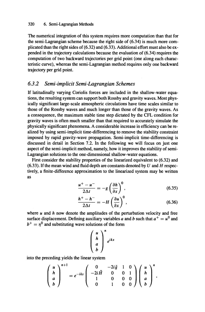
where u and h now denote the amplitudes of the perturbation velocity and free
surface displacement. Defining auxiliary variables a and b such that a+ = uo and
b+ = 71° and substituting wave solutions of the form
1
into the preceding yields the linear system
o
-2iH
o
-2ig
o
o
1
6. Semi-Lagrangian Methods
The numerical integration of this system requires more computation than that for
the semi-Lagrangian sehe me because the right side of (6.34) is much more complicated than the right sides of (6.32) and (6.33). Additional effort must also be expended in the trajectory calculations because the evaluation of (6.34) requires the
computation of two backward trajectories per grid point (one along each characteristic curve), whereas the semi-Lagrangian method requires only one backward
trajectory per grid point.
6.3.2 Semi-implicit Semi-Lagrangian Schemes
If latitudinally varying Coriolis forces are included in the shallow-water equations, the resulting system can support both Rossby and gravity waves . Most physically significant large-scale atmospheric circulations have time scales similar to
those of the Rossby waves and much longer than those of the gravity waves . As
a consequence, the maximum stable time step dictated by the CFL condition for
gravity waves is often much smaller than that required to accurately simulate the
physically significant phenomena. A considerable increase in efficiency can berealized by using semi-implicit time-differencing to remove the stability constraint
imposed by rapid gravity-wave propagation. Semi-implicit time-differencing is
discussed in detail in Section 7.2. In the following we will focus on just one
aspect of the semi-implicit method, namely, how it improves the stability of semiLagrangian solutions to the one-dimensional shallow-water equations.
First consider the stability properties of the linearized equivalent to (6.32) and
(6.33). If the mean wind and fluid depth are constants denoted by U and H respectively, a finite-difference approximation to the linearized system may be written
as
u+ - u"
2M
=-g
(6.35)
= -H (::Y
h+ -h2/lt
(6.36)
where u and h now denote the amplitudes of the perturbation velocity and free
surface displacement. Defining auxiliary variables a and b such that a+ = uo and
b+ = 71° and substituting wave solutions of the form
1
into the preceding yields the linear system
o
-2iH
o
-2ig
o
o
1