

6.2 Foreing in the Lagrangian Frame
317
"
j :'.\
\\1: 'J
'J'. ,'
"
".,
.,: ' I
. '
" I
i '{ :
'\0
!H(l/J)
\.. }
j
L
-
I '
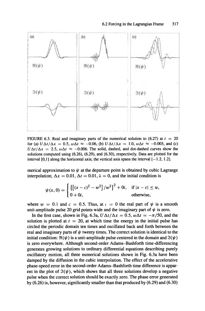
FIGDRE 6.3. Real and imaginary parts of the numerieal solution to (6.27) at I = 20
for (a) U Öl / Öx = 0 .5, wÖI -0.06, (b) U Öl / Öx = 1.0. wÖI -0.003, and (e)
U Öl / ÖX = 2.5, wÖI -0.006. The solid, dashed, and dot-dashed eurves show the
solutions eomputed using (6.26), (6.29), and (6.30), respeetively. Data are plotted for the
interval [0, I ] along the horizontal axis ; the vertical axis spans the interval [-1 .2, 1.2].
merical approximation to l/J at the departure point is obtained by cubic Lagrange
interpolation; Dox = 0.01, M = 0.01, A = 0, and the initial condition is
iflx - c]
otherwise,
w,
where w = 0.1 and c = 0.5. Thus, at I = 0 the real part of l/J is a smooth
unit-arnplitude pulse 20 grid points wide and the imaginary part of l/J is zero.
In the first case, shown in Fig. 6.3a, U Dot / Dox = 0.5, wDot = -]'{/50, and the
solution is plotted at t = 20, at which time the energy in the initial pulse has
circled the periodic domain ten times and oscillated back and forth between the
real and imaginary parts of l/J twenty times. The correct solution is identical to the
initial condition: m(l/J) is a unit-amplitude pulse centered in the domain and
is zero everywhere. Although second-order Adams-Bashforth time-differencing
generates growing solutions to ordinary differential equations describing purely
oscillatory motion, all three numerical solutions shown in Fig. 6.3a have been
damped by the diffusion in the cubic interpolation. The effect of the accelerative
phase-speed error in the second-order Adams-Bashforth time difference is apparent in the plot of
which shows that all three solutions develop a negative
pulse when the correct solution should be exactly zero. The phase error generated
by (6.26) is, however, significantly smaller than that produced by (6.29) and (6.30)
317
"
j :'.\
\\1: 'J
'J'. ,'
"
".,
.,: ' I
. '
" I
i '{ :
'\0
!H(l/J)
\.. }
j
L
-
I '
FIGDRE 6.3. Real and imaginary parts of the numerieal solution to (6.27) at I = 20
for (a) U Öl / Öx = 0 .5, wÖI -0.06, (b) U Öl / Öx = 1.0. wÖI -0.003, and (e)
U Öl / ÖX = 2.5, wÖI -0.006. The solid, dashed, and dot-dashed eurves show the
solutions eomputed using (6.26), (6.29), and (6.30), respeetively. Data are plotted for the
interval [0, I ] along the horizontal axis ; the vertical axis spans the interval [-1 .2, 1.2].
merical approximation to l/J at the departure point is obtained by cubic Lagrange
interpolation; Dox = 0.01, M = 0.01, A = 0, and the initial condition is
iflx - c]
otherwise,
w,
where w = 0.1 and c = 0.5. Thus, at I = 0 the real part of l/J is a smooth
unit-arnplitude pulse 20 grid points wide and the imaginary part of l/J is zero.
In the first case, shown in Fig. 6.3a, U Dot / Dox = 0.5, wDot = -]'{/50, and the
solution is plotted at t = 20, at which time the energy in the initial pulse has
circled the periodic domain ten times and oscillated back and forth between the
real and imaginary parts of l/J twenty times. The correct solution is identical to the
initial condition: m(l/J) is a unit-amplitude pulse centered in the domain and
is zero everywhere. Although second-order Adams-Bashforth time-differencing
generates growing solutions to ordinary differential equations describing purely
oscillatory motion, all three numerical solutions shown in Fig. 6.3a have been
damped by the diffusion in the cubic interpolation. The effect of the accelerative
phase-speed error in the second-order Adams-Bashforth time difference is apparent in the plot of
which shows that all three solutions develop a negative
pulse when the correct solution should be exactly zero. The phase error generated
by (6.26) is, however, significantly smaller than that produced by (6.29) and (6.30)