

6.2 Forcing in the Lagrangian Frame
313
A variety of other schemes have been proposed to compute back trajectories.
One popular scheme, the second-order implicit midpoint method
xi = Xj - U (Xj + xi)/2,
M ,
(6.24)
is typically solved by iteration. The Runge-Kutta scheme (6.18)-(6.19) can be
considered a two-step iterative approximation to (6.24), but even if the implicit
midpoint method is iterated to convergence, its formal order of accuracy is no
greater than that obtained using (6.18) and (6.19). A second alternative scheme
can be used if the velocities are being calculated as prognostic variables during
the integration. Then the value of dufdt can be saved after the evaluation of the
forcing terms in the momentum equation and employed in subsequent trajectory
calculations using the second-order scheme
X* = x n + 1 - u(x n + l , tn)ßt,
_
(ßt)2 du
x'! = x n + 1 - u(x tn)ßt + - - - ( x t")
J
*,
2 dt *,
(Krishnamurti et aI. 1990; Smolarkiewicz and Pudykiewicz 1992).
Higher-order schemes for the computation of back trajectories have also been
devised (Temperton and Staniforth 1987). Although a third-order trajectory scheme
must be employed as part of any fully third-order semi-Lagrangian method, higherorder trajectory computations are not widely used. In many of the applications
where semi-Lagrangian methods are most advantageous it Is easier to accurately
compute the back trajectory than it is to accurately interpolate all the resolved
scales in the tracer field. As a consequence, second-order schemes are often used
for the back trajectory calculation even when the tracer field is interpolated using cubic or higher-order polynomials. Moreover, in those problems where there
is nonzero forcing in the Lagrangian reference frame , the time integral of the
forcing is seldom approximated to more than second-order accuracy, and in such
circumstances the use of a higher-order scheme to compute the back trajectory
will not reduce the overall time-truncation error of the semi-Lagrangian scheme
below 0 [(ßt)2].
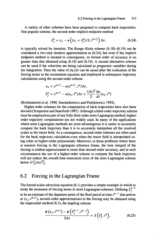
6.2 Forcing in the Lagrangian Frame
The forced scalar advection equation (6.1) provides a simple example in which to
study the treatment of forcing terms in semi-Lagrangian schemes. Defining ir
l
to be an estimate of the departure point of the fluid parcel at time t n - ) that arrives
at (xi- t n +I), second-order approximations to the forcing may be obtained using
the trapezoidal method (6.3), the leapfrog scheme
ifJ (Xj, t n + l ) - i fJ (i,!-I, tn-I)
2ßt J
= S (xi ,t
n) ,
(6.25)
313
A variety of other schemes have been proposed to compute back trajectories.
One popular scheme, the second-order implicit midpoint method
xi = Xj - U (Xj + xi)/2,
M ,
(6.24)
is typically solved by iteration. The Runge-Kutta scheme (6.18)-(6.19) can be
considered a two-step iterative approximation to (6.24), but even if the implicit
midpoint method is iterated to convergence, its formal order of accuracy is no
greater than that obtained using (6.18) and (6.19). A second alternative scheme
can be used if the velocities are being calculated as prognostic variables during
the integration. Then the value of dufdt can be saved after the evaluation of the
forcing terms in the momentum equation and employed in subsequent trajectory
calculations using the second-order scheme
X* = x n + 1 - u(x n + l , tn)ßt,
_
(ßt)2 du
x'! = x n + 1 - u(x tn)ßt + - - - ( x t")
J
*,
2 dt *,
(Krishnamurti et aI. 1990; Smolarkiewicz and Pudykiewicz 1992).
Higher-order schemes for the computation of back trajectories have also been
devised (Temperton and Staniforth 1987). Although a third-order trajectory scheme
must be employed as part of any fully third-order semi-Lagrangian method, higherorder trajectory computations are not widely used. In many of the applications
where semi-Lagrangian methods are most advantageous it Is easier to accurately
compute the back trajectory than it is to accurately interpolate all the resolved
scales in the tracer field. As a consequence, second-order schemes are often used
for the back trajectory calculation even when the tracer field is interpolated using cubic or higher-order polynomials. Moreover, in those problems where there
is nonzero forcing in the Lagrangian reference frame , the time integral of the
forcing is seldom approximated to more than second-order accuracy, and in such
circumstances the use of a higher-order scheme to compute the back trajectory
will not reduce the overall time-truncation error of the semi-Lagrangian scheme
below 0 [(ßt)2].
6.2 Forcing in the Lagrangian Frame
The forced scalar advection equation (6.1) provides a simple example in which to
study the treatment of forcing terms in semi-Lagrangian schemes. Defining ir
l
to be an estimate of the departure point of the fluid parcel at time t n - ) that arrives
at (xi- t n +I), second-order approximations to the forcing may be obtained using
the trapezoidal method (6.3), the leapfrog scheme
ifJ (Xj, t n + l ) - i fJ (i,!-I, tn-I)
2ßt J
= S (xi ,t
n) ,
(6.25)