

304
6. Semi-Lagrangian Methods
value for 1/! to each of these fluid parcels from the initial condition, and then integrate the ordinary differential equations (6.1) and (6.2) to determine the location
and the tracer concentration of each parcel as a function of time . The difficulty
with this strategy is that in most practical applications the distribution of the fluid
parcels eventually becomes highly nonuniform , and the numerical approximation
of 1/!(x, t) becomes inaccurate in regions where the fluid parcels are widely separated. In theory, this situation can be improved by adding new parcels to those
regions where the initial parcels have become widely separated and removing
parcels from regions where the parcels have become too concentrated. It is, however, difficult to create a simple algorithm for adding and removing fluid parcels
in response to their evolving distribution within the fluid.
A much better scheme for regulating the number and distribution of the fluid
parcels can be obtained by choosing a completely new set of parcels at every time
step. The parcels making up this set are those arriving at each node on a regularly spaced grid at the end of each step . As noted by Wiin-Nielsen (1959), this
approach, known as the semi -Lagrangian method, keeps the fluid parcels evenly
distributed throughout the fluid and facilitates the computation of spatial derivatives via finite differences. As an illustration of this approach, let t" = n St and
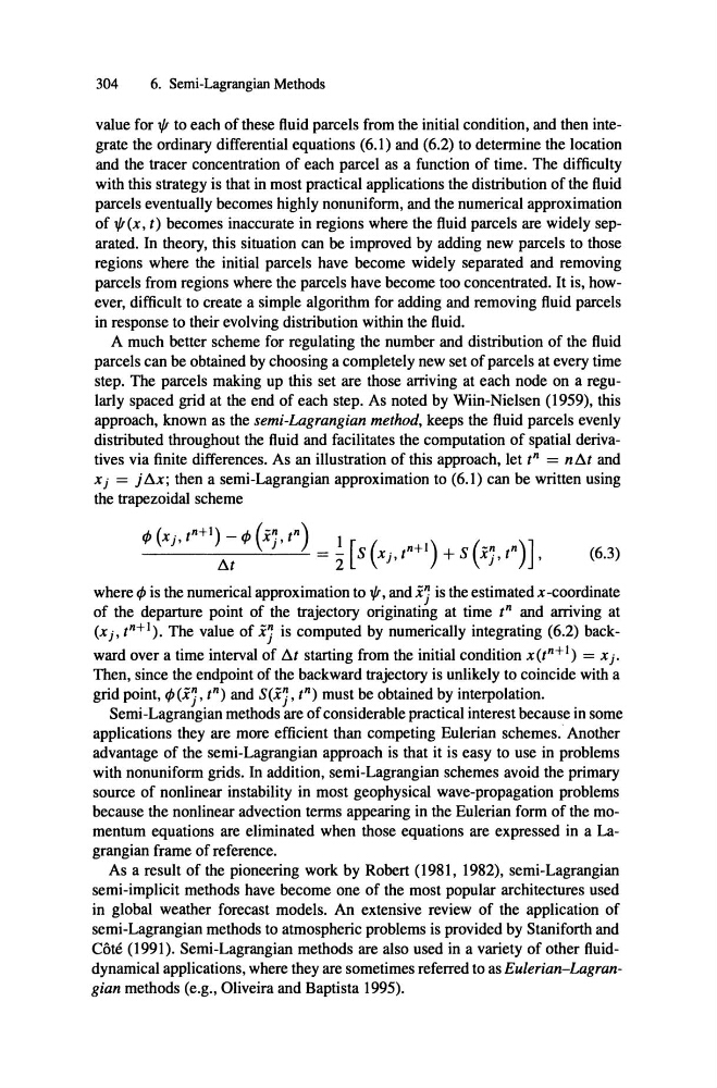
Xj = j äx; then a semi-Lagrangian approximation to (6.1) can be written using
the trapezoidal scheme
!'!.t
tP(Xj,tn+I)-tP(X'j,t
n) I [ (
S x j, t
n+l) + S x
(-n n)]
(6.3)
J
" t ,
where tP is the numerical approximation to 1/!, and x'j is the estimated x-coordinate
of the departure point of the trajectory originating at time t" and arriving at
(x], t n+ I). The value of x'j is computed by numerically integrating (6.2) backward over a time interval of !'!.t starting from the initial condition x(t n +
l ) = Xj .
Then, since the endpoint of the backward trajectory is unlikely to coincide with a
grid point, tP (x'j, t") and S(x'j, t") must be obtained by interpolation.
Semi-Lagrangian methods are of considerable practical interest because in some
applications they are more efficient than competing Eulerian schemes. Another
advantage of the semi-Lagrangian approach is that it is easy to use in problems
with nonuniform grids. In addition, semi-Lagrangian schemes avoid the primary
source of nonlinear instability in most geophysical wave-propagation problems
because the nonlinear advection terms appearing in the Eulerian form of the momentum equations are eliminated when those equations are expressed in a Lagrangian frame of reference.
As a result of the pioneering work by Robert (1981, 1982), semi-Lagrangian
semi-implicit methods have become one of the most popular architectures used
in global weather forecast models. An extensive review of the application of
semi-Lagrangian methods to atmospheric problems is provided by Staniforth and
Cöte (1991). Semi-Lagrangian methods are also used in a variety of other fluiddynamical applications, where they are sometimes referred to as Eulerian-Lagrangian methods (e.g., Oliveira and Baptista 1995).
6. Semi-Lagrangian Methods
value for 1/! to each of these fluid parcels from the initial condition, and then integrate the ordinary differential equations (6.1) and (6.2) to determine the location
and the tracer concentration of each parcel as a function of time . The difficulty
with this strategy is that in most practical applications the distribution of the fluid
parcels eventually becomes highly nonuniform , and the numerical approximation
of 1/!(x, t) becomes inaccurate in regions where the fluid parcels are widely separated. In theory, this situation can be improved by adding new parcels to those
regions where the initial parcels have become widely separated and removing
parcels from regions where the parcels have become too concentrated. It is, however, difficult to create a simple algorithm for adding and removing fluid parcels
in response to their evolving distribution within the fluid.
A much better scheme for regulating the number and distribution of the fluid
parcels can be obtained by choosing a completely new set of parcels at every time
step. The parcels making up this set are those arriving at each node on a regularly spaced grid at the end of each step . As noted by Wiin-Nielsen (1959), this
approach, known as the semi -Lagrangian method, keeps the fluid parcels evenly
distributed throughout the fluid and facilitates the computation of spatial derivatives via finite differences. As an illustration of this approach, let t" = n St and
Xj = j äx; then a semi-Lagrangian approximation to (6.1) can be written using
the trapezoidal scheme
!'!.t
tP(Xj,tn+I)-tP(X'j,t
n) I [ (
S x j, t
n+l) + S x
(-n n)]
(6.3)
J
" t ,
where tP is the numerical approximation to 1/!, and x'j is the estimated x-coordinate
of the departure point of the trajectory originating at time t" and arriving at
(x], t n+ I). The value of x'j is computed by numerically integrating (6.2) backward over a time interval of !'!.t starting from the initial condition x(t n +
l ) = Xj .
Then, since the endpoint of the backward trajectory is unlikely to coincide with a
grid point, tP (x'j, t") and S(x'j, t") must be obtained by interpolation.
Semi-Lagrangian methods are of considerable practical interest because in some
applications they are more efficient than competing Eulerian schemes. Another
advantage of the semi-Lagrangian approach is that it is easy to use in problems
with nonuniform grids. In addition, semi-Lagrangian schemes avoid the primary
source of nonlinear instability in most geophysical wave-propagation problems
because the nonlinear advection terms appearing in the Eulerian form of the momentum equations are eliminated when those equations are expressed in a Lagrangian frame of reference.
As a result of the pioneering work by Robert (1981, 1982), semi-Lagrangian
semi-implicit methods have become one of the most popular architectures used
in global weather forecast models. An extensive review of the application of
semi-Lagrangian methods to atmospheric problems is provided by Staniforth and
Cöte (1991). Semi-Lagrangian methods are also used in a variety of other fluiddynamical applications, where they are sometimes referred to as Eulerian-Lagrangian methods (e.g., Oliveira and Baptista 1995).