

286
5. Finite-Volume Methods
y
o
x
.......
... i
x
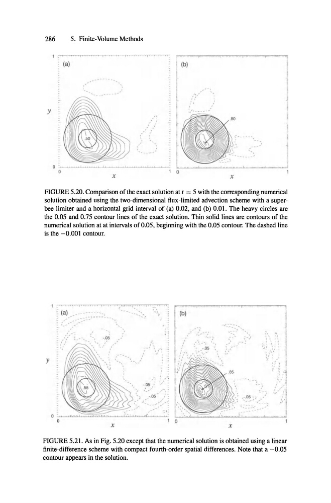
FIGURE 5.20. Comparison ofthe exact solution at t = 5 with the corresponding numerical
solution obtained using the two-dirnensional flux-limited advection scheme with a superbee limiter and a horizontal grid interval of (a) 0.02, and (b) 0.01. The heavy circles are
the 0.05 and 0.75 contour lines of the exact solution. Thin solid lines are contours of the
numerical solution at at intervals ofO.05, beginning with the 0.05 contour. The dashed line
is the -0.001 contour.
..
-
,
1
.",
.
, . ,
'"
'- ,
" ,
: ."
· .'
· ,','
.....
..
y
.',:'" ...
x
l
: .....
... ..
.. '
, .'
'.
.:
"
,' :
' " i
',. '" ;: I
.: ,
' <:.1 " ;
•
,".) :
•
I
I
"i
,
x
FIGURE 5.21. As in Fig. 5.20 except that the numerical solution is obtained using a linear
finite-difference scheme with compact fourth -order spatial differences . Note that a -0.05
contour appears in the solution.
5. Finite-Volume Methods
y
o
x
.......
... i
x
FIGURE 5.20. Comparison ofthe exact solution at t = 5 with the corresponding numerical
solution obtained using the two-dirnensional flux-limited advection scheme with a superbee limiter and a horizontal grid interval of (a) 0.02, and (b) 0.01. The heavy circles are
the 0.05 and 0.75 contour lines of the exact solution. Thin solid lines are contours of the
numerical solution at at intervals ofO.05, beginning with the 0.05 contour. The dashed line
is the -0.001 contour.
..
-
,
1
.",
.
, . ,
'"
'- ,
" ,
: ."
· .'
· ,','
.....
..
y
.',:'" ...
x
l
: .....
... ..
.. '
, .'
'.
.:
"
,' :
' " i
',. '" ;: I
.: ,
' <:.1 " ;
•
,".) :
•
I
I
"i
,
x
FIGURE 5.21. As in Fig. 5.20 except that the numerical solution is obtained using a linear
finite-difference scheme with compact fourth -order spatial differences . Note that a -0.05
contour appears in the solution.