

284
5. Finite-Volume Methods
F" 1 , = 0,
I-'Z ,)
G? , I = 0,
I ,)-'Z
!i.'! , = 0,
I .)
!i.'! , = !i.'! ,+U(4JI+l )' - 4JI )'),
I ,)
I ,)
(*)
(**)
4J;+) '
,
"
1
= 4J'i)' - !i.t (!i.j), + F,n+ 1 , - F.
n I ,+ G? '+ 1 - G? , I] '
I 'Z')
I-'Z,)
I ,) 'Z
I,)-'Z
'
!i.s
'
(***)
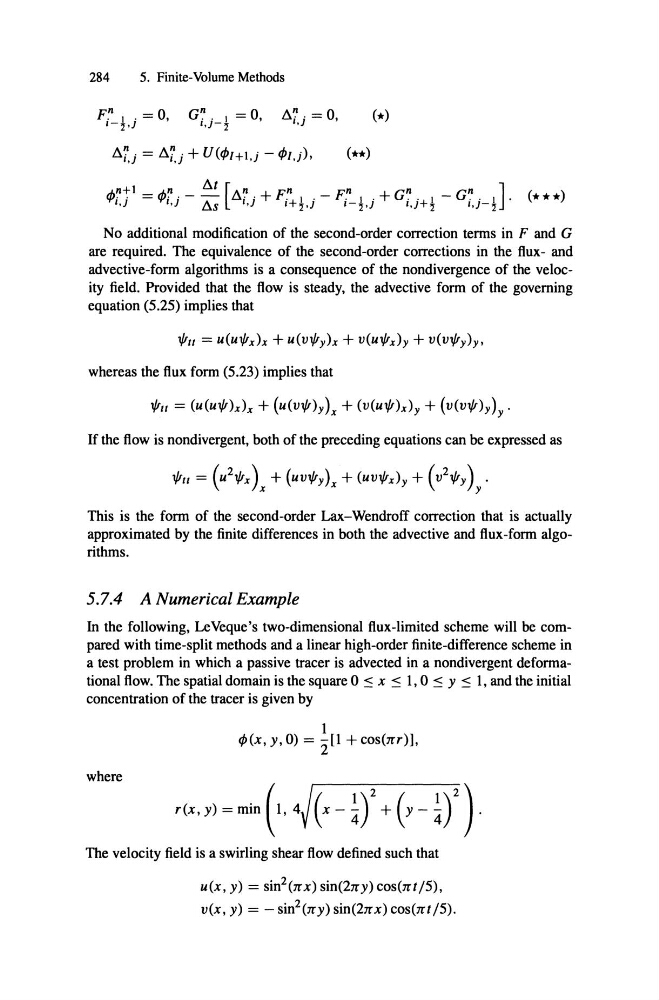
No additional modification of the second-order correction terms in F and G
are required. The equivalence of the second-order corrections in the flux- and
advective-form algorithms is a consequence of the nondivergence of the velocity field. Provided that the flow is steady, the advective form of the goveming
equation (5.25) implies that
whereas the flux form (5.23) implies that
If the flow is nondivergent, both of the preceding equations can be expressed as
tional flow. The spatial domain is the square 0
concentration of the tracer is given by
x
1, 0 s Y 1, and the initial
This is the form of the second-order Lax-Wendroff correction that is actually
approximated by the finite differences in both the advective and flux-form algorithms.
5.7.4 A Numerical Example
In the following , LeVeque's two-dimensional flux-limited scheme will be compared with time-split methods and a linear high-order finite-difference scheme in
a test problem in which a passive tracer is advected in a nondivergent deformaI
4J(x, y , 0) = 2[1 + cos(rrr)],
where
The velocity field is a swirling shear flow defined such that
u(x, y) = sin
2(rrx) sin(2rry) cos(rrt/5) ,
v( x, y) = - sin
2(rry) sin(2rr x) cos(rrt /5) .
5. Finite-Volume Methods
F" 1 , = 0,
I-'Z ,)
G? , I = 0,
I ,)-'Z
!i.'! , = 0,
I .)
!i.'! , = !i.'! ,+U(4JI+l )' - 4JI )'),
I ,)
I ,)
(*)
(**)
4J;+) '
,
"
1
= 4J'i)' - !i.t (!i.j), + F,n+ 1 , - F.
n I ,+ G? '+ 1 - G? , I] '
I 'Z')
I-'Z,)
I ,) 'Z
I,)-'Z
'
!i.s
'
(***)
No additional modification of the second-order correction terms in F and G
are required. The equivalence of the second-order corrections in the flux- and
advective-form algorithms is a consequence of the nondivergence of the velocity field. Provided that the flow is steady, the advective form of the goveming
equation (5.25) implies that
whereas the flux form (5.23) implies that
If the flow is nondivergent, both of the preceding equations can be expressed as
tional flow. The spatial domain is the square 0
concentration of the tracer is given by
x
1, 0 s Y 1, and the initial
This is the form of the second-order Lax-Wendroff correction that is actually
approximated by the finite differences in both the advective and flux-form algorithms.
5.7.4 A Numerical Example
In the following , LeVeque's two-dimensional flux-limited scheme will be compared with time-split methods and a linear high-order finite-difference scheme in
a test problem in which a passive tracer is advected in a nondivergent deformaI
4J(x, y , 0) = 2[1 + cos(rrr)],
where
The velocity field is a swirling shear flow defined such that
u(x, y) = sin
2(rrx) sin(2rry) cos(rrt/5) ,
v( x, y) = - sin
2(rry) sin(2rr x) cos(rrt /5) .