

1.2 Wave Equations in Geophysical Fluid Dynamies
13
fluctuations in 1{! occur on much smaller scales than those of primary interest in
most geophysical problems. Thus in most geophysical applications the solution to
CI .24) is essentially identical to that for the inviscid problem, and the numerical
techniques suitable for the approximation of (1.24) are almost identical to those
for the purely hyperbolic problem (1.22).
When computing numerical solutions to either (1.22) or (1.24), there will be
limits on the spatial and temporal scales at which the velocity field can be rep -
resented in any finite data set. The influence of the unresolved velocity perturbations on the distribution of the tracer is not directly computable, but is often
parametrized by replacing K by an eddy dijfusivity, K e • The eddy diffusivity is
supposed to represent the tendency of random unresolved velocity fluctuations to
spread the distribution of 1{! away from the centerline of the smooth air-parcel trajectories computed from the resolved-scale velocity field. Eddy diffusivities are
much larger than the molecular diffusivity, but even when K is replaced by a typical eddy diffusivity, the terms on the right side of CI .22) remain relatively smalI,
and the basic character of the solution is still wave-like. Nevertheless, some eddy -
diffusivity parametrizations do generate large values for K e in limited regions of
the flow. High values of K e might, for example, be found in the planetary boundary
layer where strong subgrid-scale motions are driven by thermal and mechanical
turbulence. Large K e might also be parametrized to develop in regions where vigorous subgrid-scale motions are generated through Kelvin-Helmholtz instability.
In these limited areas of high eddy diffusivity, the solutions to the parametrized
problem may no longer be wave-like.
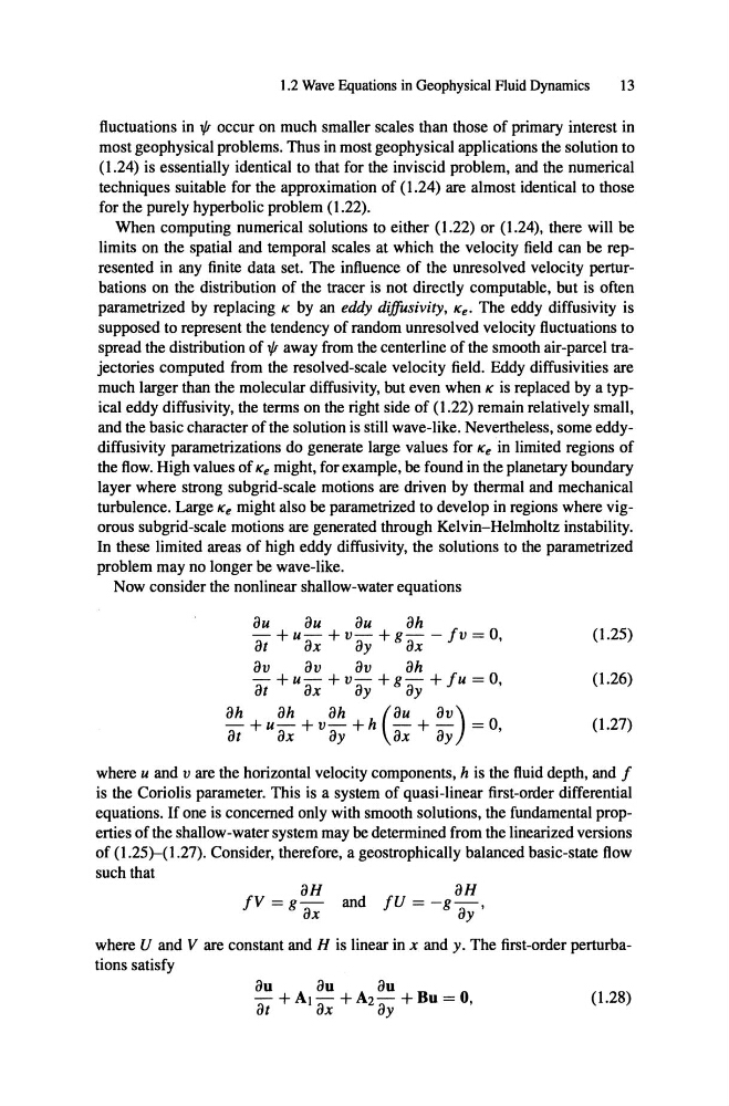
Now consider the nonlinear shallow-water equations
8u
8u
8u
8h
- + u- + v- + g - - f » = 0,
8t
8x
8y
8x
8v
8v
8v
8h
- +u - +v- +g- + f u =0,
8t
8x
8y
8y
-+u-+v-+h 8h
8h
8h
(8U -+- 8V) =0,
8t
8x
8y
8x
8y
(1.25)
(1.26)
(1.27)
where u and v are the horizontal velocity components, h is the fluid depth, and I
is the Coriolis parameter. This is a system of quasi-linear first-order differential
equations. If one is concemed only with smooth solutions, the fundamental properties of the shallow-water system may be determined from the linearized versions
of (1.25)-(1.27). Consider, therefore, a geostrophically balanced basic-state flow
such that
8H
IV=g- and
8H
IU = - g - ,
where U and V are constant and H is linear in x and y . The first-order perturbations satisfy
8u
8u
8u
-+A\-+A2 - +Bu=O,
8t
8x
8y
(1.28)
13
fluctuations in 1{! occur on much smaller scales than those of primary interest in
most geophysical problems. Thus in most geophysical applications the solution to
CI .24) is essentially identical to that for the inviscid problem, and the numerical
techniques suitable for the approximation of (1.24) are almost identical to those
for the purely hyperbolic problem (1.22).
When computing numerical solutions to either (1.22) or (1.24), there will be
limits on the spatial and temporal scales at which the velocity field can be rep -
resented in any finite data set. The influence of the unresolved velocity perturbations on the distribution of the tracer is not directly computable, but is often
parametrized by replacing K by an eddy dijfusivity, K e • The eddy diffusivity is
supposed to represent the tendency of random unresolved velocity fluctuations to
spread the distribution of 1{! away from the centerline of the smooth air-parcel trajectories computed from the resolved-scale velocity field. Eddy diffusivities are
much larger than the molecular diffusivity, but even when K is replaced by a typical eddy diffusivity, the terms on the right side of CI .22) remain relatively smalI,
and the basic character of the solution is still wave-like. Nevertheless, some eddy -
diffusivity parametrizations do generate large values for K e in limited regions of
the flow. High values of K e might, for example, be found in the planetary boundary
layer where strong subgrid-scale motions are driven by thermal and mechanical
turbulence. Large K e might also be parametrized to develop in regions where vigorous subgrid-scale motions are generated through Kelvin-Helmholtz instability.
In these limited areas of high eddy diffusivity, the solutions to the parametrized
problem may no longer be wave-like.
Now consider the nonlinear shallow-water equations
8u
8u
8u
8h
- + u- + v- + g - - f » = 0,
8t
8x
8y
8x
8v
8v
8v
8h
- +u - +v- +g- + f u =0,
8t
8x
8y
8y
-+u-+v-+h 8h
8h
8h
(8U -+- 8V) =0,
8t
8x
8y
8x
8y
(1.25)
(1.26)
(1.27)
where u and v are the horizontal velocity components, h is the fluid depth, and I
is the Coriolis parameter. This is a system of quasi-linear first-order differential
equations. If one is concemed only with smooth solutions, the fundamental properties of the shallow-water system may be determined from the linearized versions
of (1.25)-(1.27). Consider, therefore, a geostrophically balanced basic-state flow
such that
8H
IV=g- and
8H
IU = - g - ,
where U and V are constant and H is linear in x and y . The first-order perturbations satisfy
8u
8u
8u
-+A\-+A2 - +Bu=O,
8t
8x
8y
(1.28)