

176
4. Series-Expansion Methods
coefficients of the form
where
lnk = ({Jn({Jk dx.
The initial conditions for the preceding system of differential equations are obtained by choosing al (to), .. . , aN(to) such that r!J(x, to) provides the "best" approximation to [tx) . The possible strategies for constraining the initial error are
identical to those used to ensure that the residual is srnall. As before, the choice
that minimizes the tz-nonn of the initial error also satisfies the Galerkin requirement that the initial error be orthogonal to each of the expansion functions,
- !(X)) ({Jk(X) dx = 0 for an k = I, . . . , N,
or, equivalently,
N
L lnkan = [ !(X)({Jk(X) dx for an k = I, . . . , N.
n=1
ls
(4.8)
4.2 The Spectral Method
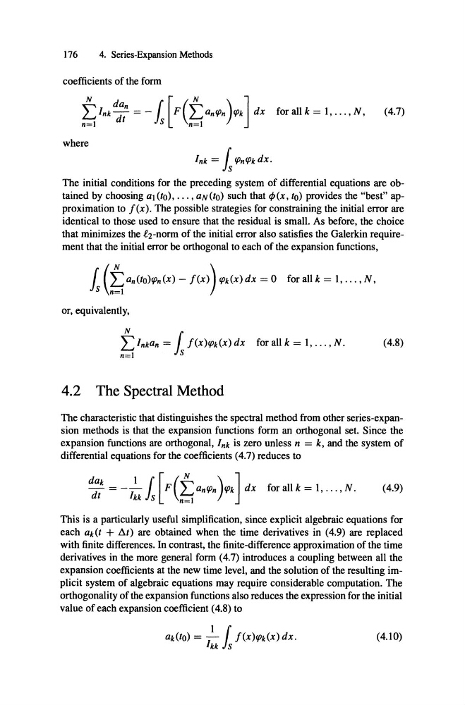
The characteristic that distinguishes the spectral method from other series-expansion methods is that the expansion functions form an orthogonal set. Since the
expansion functions are orthogonal, lnk is zero unless n = k, and the system of
differential equations for the coefficients (4.7) reduces to
dak = __ 1 [ [F (t an({Jn)({Jk] dx for an k = 1, .. . , N. (4.9)
dt
lkk Js n=1
This is a particularly useful simplification, since explicit algebraic equations for
each ak(t +
are obtained when the time derivatives in (4.9) are replaced
with finite differences. In contrast , the finite-difference approximation of the time
derivatives in the more general form (4.7) introduces a coupling between an the
expansion coefficients at the new time level, and the solution of the resulting implicit system of algebraic equations may require considerable computation . The
orthogonality of the expansion functions also reduces the expression for the initial
value of each expansion coefficient (4.8) to
(4.10)
4. Series-Expansion Methods
coefficients of the form
where
lnk = ({Jn({Jk dx.
The initial conditions for the preceding system of differential equations are obtained by choosing al (to), .. . , aN(to) such that r!J(x, to) provides the "best" approximation to [tx) . The possible strategies for constraining the initial error are
identical to those used to ensure that the residual is srnall. As before, the choice
that minimizes the tz-nonn of the initial error also satisfies the Galerkin requirement that the initial error be orthogonal to each of the expansion functions,
- !(X)) ({Jk(X) dx = 0 for an k = I, . . . , N,
or, equivalently,
N
L lnkan = [ !(X)({Jk(X) dx for an k = I, . . . , N.
n=1
ls
(4.8)
4.2 The Spectral Method
The characteristic that distinguishes the spectral method from other series-expansion methods is that the expansion functions form an orthogonal set. Since the
expansion functions are orthogonal, lnk is zero unless n = k, and the system of
differential equations for the coefficients (4.7) reduces to
dak = __ 1 [ [F (t an({Jn)({Jk] dx for an k = 1, .. . , N. (4.9)
dt
lkk Js n=1
This is a particularly useful simplification, since explicit algebraic equations for
each ak(t +
are obtained when the time derivatives in (4.9) are replaced
with finite differences. In contrast , the finite-difference approximation of the time
derivatives in the more general form (4.7) introduces a coupling between an the
expansion coefficients at the new time level, and the solution of the resulting implicit system of algebraic equations may require considerable computation . The
orthogonality of the expansion functions also reduces the expression for the initial
value of each expansion coefficient (4.8) to
(4.10)