

3.5 Linear Equations with Variable Coefficients
155
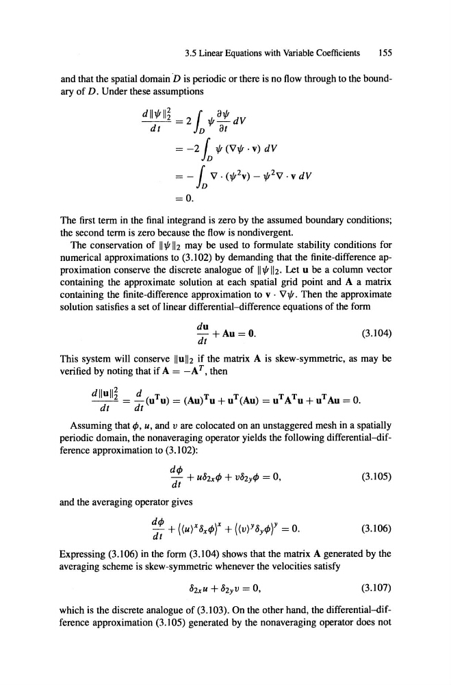
and that the spatial domain 'D is pcriodie or there is no flow through to the boundary of D. Under these assumptions
= 2 { 1/1 a1/l dV
dt
10 at
= -2L1/I (V1/I . v) dV
= -L v· (1/I2v) - 1/I2V . v dV
=0.
The first term in the final integrand is zero by the assumed boundary eonditions;
the seeond term is zero beeause the flow is nondivergent.
The eonservation of 111/1 112 may be used to formulate stability eonditions for
numerical approximations to (3.102) by demanding that the finite-differenee approximation eonserve the diserete analogue of 111/1112. Let u be a eolumn veetor
eontaining the approximate solution at eaeh spatial grid point and A a matrix
eontaining the finite-differenee approximation to v . V1/1 . Then the approximate
solution satisfies a set of linear differential-differenee equations of the form
du
-+Au=O.
dt
(3.104)
This system will eonserve lIull2 if the matrix A is skew-symrnetric, as may be
verified by noting that if A = -AT, then
Assuming that cf> , u, and v are colocated on an unstaggered mesh in a spatially
periodic domain, the nonaveraging operator yields the following differential-differenee approximation to (3.102):
(3.105)
and the averaging operator gives
dcf> + ((u)X oxcf»X + ((v)Y Oycf» Y = O.
dt
(3.106)
Expressing (3.106) in the form (3.104) shows that the matrix A generated by the
averaging sehe me is skew-symmetrie whenever the velocities satisfy
(3.107)
whieh is the diserete analogue of (3.103). On the other hand , the differential-difference approximation (3.105) generated by the nonaveraging operator does not
155
and that the spatial domain 'D is pcriodie or there is no flow through to the boundary of D. Under these assumptions
= 2 { 1/1 a1/l dV
dt
10 at
= -2L1/I (V1/I . v) dV
= -L v· (1/I2v) - 1/I2V . v dV
=0.
The first term in the final integrand is zero by the assumed boundary eonditions;
the seeond term is zero beeause the flow is nondivergent.
The eonservation of 111/1 112 may be used to formulate stability eonditions for
numerical approximations to (3.102) by demanding that the finite-differenee approximation eonserve the diserete analogue of 111/1112. Let u be a eolumn veetor
eontaining the approximate solution at eaeh spatial grid point and A a matrix
eontaining the finite-differenee approximation to v . V1/1 . Then the approximate
solution satisfies a set of linear differential-differenee equations of the form
du
-+Au=O.
dt
(3.104)
This system will eonserve lIull2 if the matrix A is skew-symrnetric, as may be
verified by noting that if A = -AT, then
Assuming that cf> , u, and v are colocated on an unstaggered mesh in a spatially
periodic domain, the nonaveraging operator yields the following differential-differenee approximation to (3.102):
(3.105)
and the averaging operator gives
dcf> + ((u)X oxcf»X + ((v)Y Oycf» Y = O.
dt
(3.106)
Expressing (3.106) in the form (3.104) shows that the matrix A generated by the
averaging sehe me is skew-symmetrie whenever the velocities satisfy
(3.107)
whieh is the diserete analogue of (3.103). On the other hand , the differential-difference approximation (3.105) generated by the nonaveraging operator does not