

3.2 Three or More Independent Variables
127
um+ . . !. . . . n
2
v
w m . n ++
um- 1.n
r.: bm•n
tJ.z
1
T
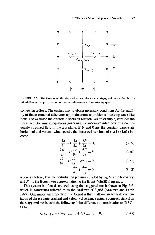
FIGURE 3.6. Distribution of the dependent variables on a staggered mesh for the finite-difference approximation of the two-dimensional Boussinesq system.
somewhat tedious. The easiest way to obtain necessary conditions for the stability of linear centered-difference approximations to problems involving wave-like
flow is to examine the discrete dispersion relation. As an example, consider the
Iinearized Boussinesq equations goveming the incompressible flow of a continuously stratified fluid in the x-z plane. If U and °are the constant basic-state
horizontal and vertical wind speeds, the linearized versions of (1.61)-(1.63) become
OU
- ot + U -
OU
OX
oP
+ - OX
= 0,
ow
-
ot
+ U -
ow
OX
oP
+ -
oz
= b
ob
- ot + U -
ob
+ N
2 w = 0,
OX
OU + OW _ °
OX
oz - ,
(3.39)
(3.40)
(3.41)
(3.42)
where as before, P is the perturbation pressure divided by Po , b is the buoyancy,
and N 2 is the Boussinesq approximation to the Brunt-Väisälä frequency.
This system is often discretized using the staggered mesh shown in Fig. 3.6,
which is sometimes referred to as the Arakawa "C" grid (Arakawa and Lamb
1977). One important property of the C-grid is that it allows an accurate computation of the pressure gradient and velocity divergence using a compact stencil on
the staggered mesh, as in the following finite-difference approximation to (3.39)(3.42)
(3.43)
127
um+ . . !. . . . n
2
v
w m . n ++
um- 1.n
r.: bm•n
tJ.z
1
T
FIGURE 3.6. Distribution of the dependent variables on a staggered mesh for the finite-difference approximation of the two-dimensional Boussinesq system.
somewhat tedious. The easiest way to obtain necessary conditions for the stability of linear centered-difference approximations to problems involving wave-like
flow is to examine the discrete dispersion relation. As an example, consider the
Iinearized Boussinesq equations goveming the incompressible flow of a continuously stratified fluid in the x-z plane. If U and °are the constant basic-state
horizontal and vertical wind speeds, the linearized versions of (1.61)-(1.63) become
OU
- ot + U -
OU
OX
oP
+ - OX
= 0,
ow
-
ot
+ U -
ow
OX
oP
+ -
oz
= b
ob
- ot + U -
ob
+ N
2 w = 0,
OX
OU + OW _ °
OX
oz - ,
(3.39)
(3.40)
(3.41)
(3.42)
where as before, P is the perturbation pressure divided by Po , b is the buoyancy,
and N 2 is the Boussinesq approximation to the Brunt-Väisälä frequency.
This system is often discretized using the staggered mesh shown in Fig. 3.6,
which is sometimes referred to as the Arakawa "C" grid (Arakawa and Lamb
1977). One important property of the C-grid is that it allows an accurate computation of the pressure gradient and velocity divergence using a compact stencil on
the staggered mesh, as in the following finite-difference approximation to (3.39)(3.42)
(3.43)