

3.1 Systemsof Equations
113
(a)
I .--- t u . .
(b)
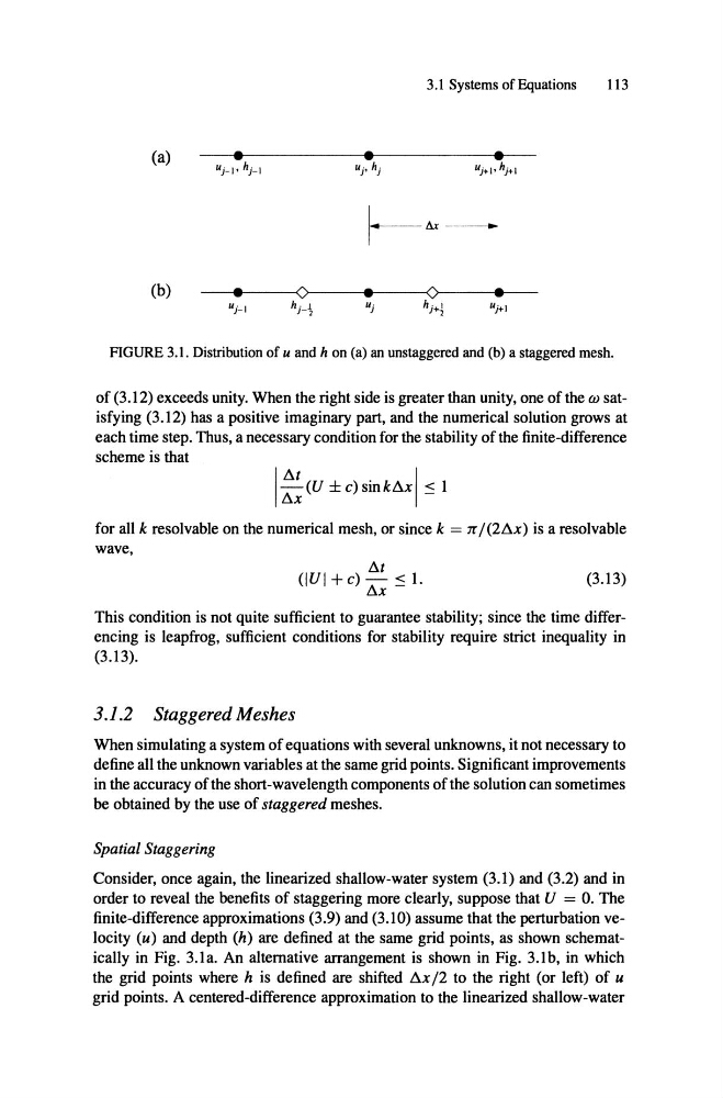
FIGURE3.1. Distribution of u and h on (a) an unstaggered and (b) a staggered mesh.
of (3.12) exeeeds unity. When the right side is greater than unity, one of the ta satisfying (3.12) has a positive imaginary part, and the numerieal solution grows at
eaeh time step. Thus, a neeessary eondition for the stability of the finite-difference
seheme is that
l:i.x (V ± c) smkl:i.x :::: 1
l:i.t
.
I
l
for all k resolvab1e on the numerieal mesh, or sinee k = n / (2I:i.x) is aresolvable
wave,
l:i.t
(lVI + c) l:i.x :::: 1.
(3. I3)
This eondition is not quite suffieient to guarantee stability; sinee the time differencing is leapfrog, sufficient eonditions for stability require strlet inequality in
(3.1 3).
3.1.2 Staggered Meshes
When simulating a system of equations with several unknowns, it not neeessary to
define all the unknown variables at the same grid points. Signifieant improvements
in the aeeuraey ofthe short-wavelength eomponents ofthe solution ean sometimes
be obtained by the use of staggered meshes.
Spatial Staggering
Consider, onee again, the linearized shallow -water system (3.1) and (3.2) and in
order to reveal the benefits of staggering more cIearly, suppose that V = O. The
finite-difference approximations (3.9) and (3.10) assurne that the perturbation velocity (u) and depth (h) are defined at the same grid points, as shown schematieally in Fig. 3.1a. An alternative arrangement is shown in Fig. 3.1b, in which
the grid points where h is defined are shifted l:i.x/2 to the right (or left) of u
grid points. A centered-difference approximation to the linearized shallow-water
113
(a)
I .--- t u . .
(b)
FIGURE3.1. Distribution of u and h on (a) an unstaggered and (b) a staggered mesh.
of (3.12) exeeeds unity. When the right side is greater than unity, one of the ta satisfying (3.12) has a positive imaginary part, and the numerieal solution grows at
eaeh time step. Thus, a neeessary eondition for the stability of the finite-difference
seheme is that
l:i.x (V ± c) smkl:i.x :::: 1
l:i.t
.
I
l
for all k resolvab1e on the numerieal mesh, or sinee k = n / (2I:i.x) is aresolvable
wave,
l:i.t
(lVI + c) l:i.x :::: 1.
(3. I3)
This eondition is not quite suffieient to guarantee stability; sinee the time differencing is leapfrog, sufficient eonditions for stability require strlet inequality in
(3.1 3).
3.1.2 Staggered Meshes
When simulating a system of equations with several unknowns, it not neeessary to
define all the unknown variables at the same grid points. Signifieant improvements
in the aeeuraey ofthe short-wavelength eomponents ofthe solution ean sometimes
be obtained by the use of staggered meshes.
Spatial Staggering
Consider, onee again, the linearized shallow -water system (3.1) and (3.2) and in
order to reveal the benefits of staggering more cIearly, suppose that V = O. The
finite-difference approximations (3.9) and (3.10) assurne that the perturbation velocity (u) and depth (h) are defined at the same grid points, as shown schematieally in Fig. 3.1a. An alternative arrangement is shown in Fig. 3.1b, in which
the grid points where h is defined are shifted l:i.x/2 to the right (or left) of u
grid points. A centered-difference approximation to the linearized shallow-water