

108
3. Beyond the One-Way Wave Equation
in which U and u(x, t) represent the mean and perturbation fluid velocity, H
and h (x , t) are the mean and perturbation fluid depth, and g is the gravitational
acceleration. The procedure for determining the truncation error, consistency, and
order of accuracy of finite-difference approximations to a system such as (3.1)
and (3.2) is identical to that discussed in Section 2.1. Taylor series expansions
for the exact solution at the various grid points (xQ, XQ ± Llx , . . .) are substituted
into each finite difference, and the order of accuracy of the overall scheme is
determined by the lowest powers of tu and Llt appearing in the truncation error.
The stability analysis for finite-difference approximations to systems of partial
differential equations is, on the other hand, more complex than that for a single
equation.
3.1.1 Stability
Recall that a Von Neumann stability analysis of the finite-difference approximation to a linear constant-coefficient scalar equation is performed by determining
the magnitude of the amplification factor Ak. Here , as in Section 2.2.2, the amplification factor for a two-time-level scheme is defined such that a single step
of the finite-difference integration maps the Fourier component e ikx to Akeikx.
However, when the goveming equations are approximated by a linear constantcoefficient system of finite-difference equations, the kth Fourier component of
the solution is represented by the vector Vb and the amplification factor becomes
an amplification matrix Ak . For example, in the shallow-water system (3.1) and
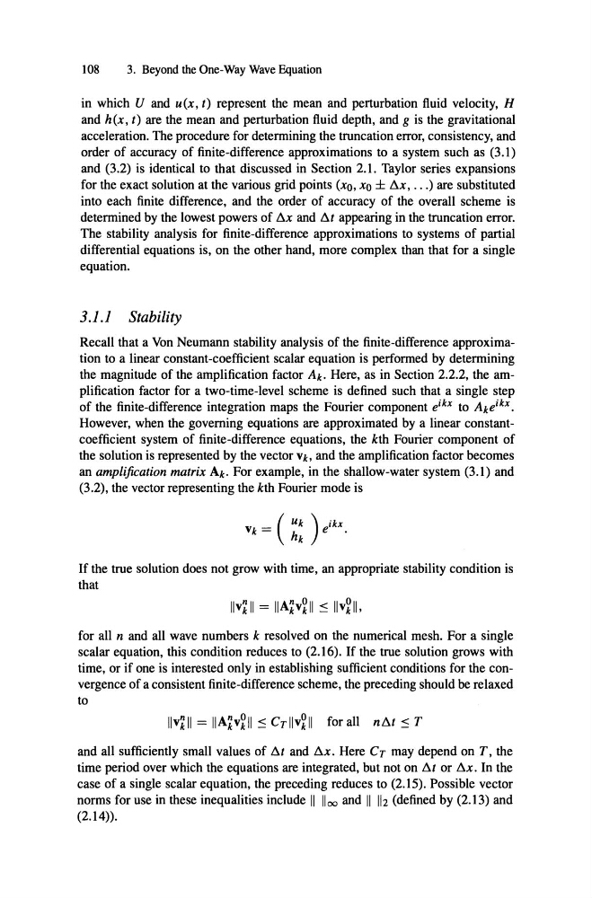
(3.2), the vector representing the kth Fourier mode is
If the true solution does not grow with time, an appropriate stability condition is
that
for a11 n and a11 wave numbers k resolved on the numerical mesh. For a single
scalar equation, this condition reduces to (2.16) . If the true solution grows with
time, or if one is interested only in establishing sufficient conditions for the con -
vergence of a consistent finite -difference scheme, the preceding should be relaxed
to
and all sufficiently small values of Llt and Sx, Here Cr may depend on T, the
time period over which the equations are integrated, but not on Llt or Sx, In the
case of a single scalar equation, the preceding reduces to (2.15) . Possible vector
norms for use in these inequalities include 11 1100 and 11 112 (defined by (2.13) and
(2.14» .
3. Beyond the One-Way Wave Equation
in which U and u(x, t) represent the mean and perturbation fluid velocity, H
and h (x , t) are the mean and perturbation fluid depth, and g is the gravitational
acceleration. The procedure for determining the truncation error, consistency, and
order of accuracy of finite-difference approximations to a system such as (3.1)
and (3.2) is identical to that discussed in Section 2.1. Taylor series expansions
for the exact solution at the various grid points (xQ, XQ ± Llx , . . .) are substituted
into each finite difference, and the order of accuracy of the overall scheme is
determined by the lowest powers of tu and Llt appearing in the truncation error.
The stability analysis for finite-difference approximations to systems of partial
differential equations is, on the other hand, more complex than that for a single
equation.
3.1.1 Stability
Recall that a Von Neumann stability analysis of the finite-difference approximation to a linear constant-coefficient scalar equation is performed by determining
the magnitude of the amplification factor Ak. Here , as in Section 2.2.2, the amplification factor for a two-time-level scheme is defined such that a single step
of the finite-difference integration maps the Fourier component e ikx to Akeikx.
However, when the goveming equations are approximated by a linear constantcoefficient system of finite-difference equations, the kth Fourier component of
the solution is represented by the vector Vb and the amplification factor becomes
an amplification matrix Ak . For example, in the shallow-water system (3.1) and
(3.2), the vector representing the kth Fourier mode is
If the true solution does not grow with time, an appropriate stability condition is
that
for a11 n and a11 wave numbers k resolved on the numerical mesh. For a single
scalar equation, this condition reduces to (2.16) . If the true solution grows with
time, or if one is interested only in establishing sufficient conditions for the con -
vergence of a consistent finite -difference scheme, the preceding should be relaxed
to
and all sufficiently small values of Llt and Sx, Here Cr may depend on T, the
time period over which the equations are integrated, but not on Llt or Sx, In the
case of a single scalar equation, the preceding reduces to (2.15) . Possible vector
norms for use in these inequalities include 11 1100 and 11 112 (defined by (2.13) and
(2.14» .