

94
2. Basic Finite-Difference Methods
may be obtained after dividing (2.98) by (2.97). The function arctan Wrl:i.t is
single-valued over the range of resolvable frequencies 0 S Wr S n / l:i.t, so as
expected for a two-time-level scheme, there is no computational mode. In the
limit of good numerical resolution,
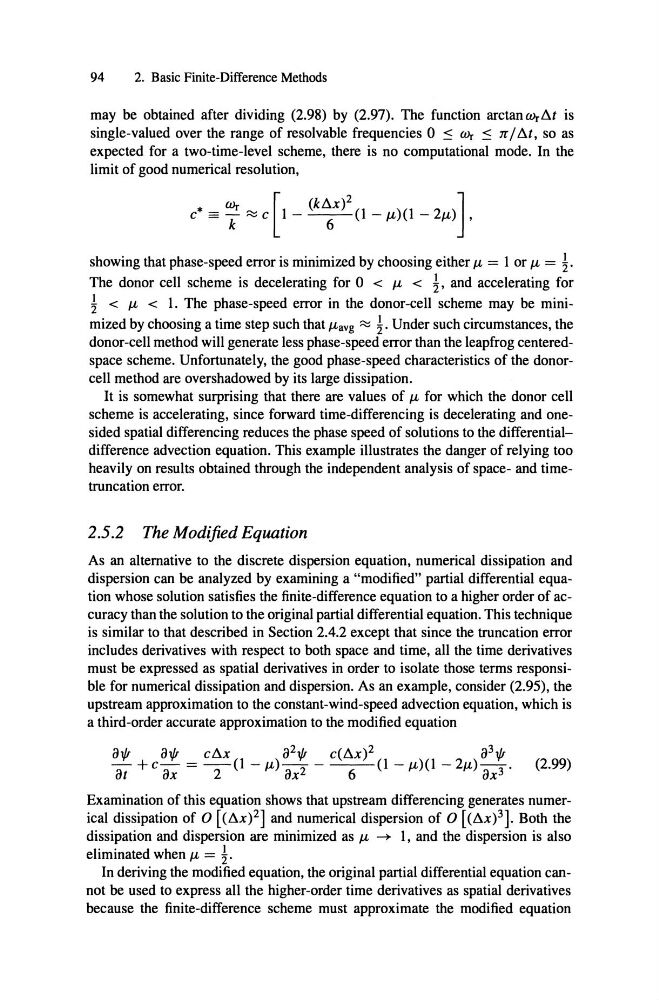
showing that phase-speed error is minimized by choosing either I-t = I or I-t = !.
The donor cell scheme is decelerating for 0 < I-t < !, and accelerating for
! < I-t < I. The phase-speed error in the donor-cell scheme may be minimized by choosing a time step such that I-tavg
Under such circumstances, the
donor-cell method will generate less phase-speed error than the leapfrog centeredspace scheme. Unfortunately, the good phase-speed characteristics of the donorcell method are overshadowed by its large dissipation.
It is somewhat surprising that there are values of I-t for which the donor cell
scheme is accelerating, since forward time-differencing is decelerating and onesided spatial differencing reduces the phase speed of solutions to the differentialdifference advection equation. This example illustrates the danger of relying too
heavily on results obtained through the independent analysis of space- and timetruncation error.
2.5.2 The Modified Equation
As an alternative to the discrete dispersion equation, numerical dissipation and
dispersion can be analyzed by examining a "modified" partial differential equation whose solution satisfies the finite-difference equation to a higher order of accuracy than the solution to the original partial differential equation . This technique
is similar to that described in Section 2.4.2 except that since the truncation error
includes derivatives with respect to both space and time, all the time derivatives
must be expressed as spatial derivatives in order to isolate those terms responsi -
ble for numerical dissipation and dispersion . As an example, consider (2.95), the
upstream approximation to the constant-wind-speed advection equation , which is
a third-order accurate approximation to the modified equation
Examination of this equation shows that upstream differencing generates numerical dissipation of 0 [(l:i.x)2] and numerical dispersion of 0 [(l:i.x)3]. Both the
dissipation and dispersion are minimized as I-t ---+
eliminated when JL = !.
I, and the dispersion is also
In deriving the modified equation, the original partial differential equation cannot be used to express all the higher-order time derivatives as spatial derivatives
because the finite-difference scheme must approximate the modified equation
2. Basic Finite-Difference Methods
may be obtained after dividing (2.98) by (2.97). The function arctan Wrl:i.t is
single-valued over the range of resolvable frequencies 0 S Wr S n / l:i.t, so as
expected for a two-time-level scheme, there is no computational mode. In the
limit of good numerical resolution,
showing that phase-speed error is minimized by choosing either I-t = I or I-t = !.
The donor cell scheme is decelerating for 0 < I-t < !, and accelerating for
! < I-t < I. The phase-speed error in the donor-cell scheme may be minimized by choosing a time step such that I-tavg
Under such circumstances, the
donor-cell method will generate less phase-speed error than the leapfrog centeredspace scheme. Unfortunately, the good phase-speed characteristics of the donorcell method are overshadowed by its large dissipation.
It is somewhat surprising that there are values of I-t for which the donor cell
scheme is accelerating, since forward time-differencing is decelerating and onesided spatial differencing reduces the phase speed of solutions to the differentialdifference advection equation. This example illustrates the danger of relying too
heavily on results obtained through the independent analysis of space- and timetruncation error.
2.5.2 The Modified Equation
As an alternative to the discrete dispersion equation, numerical dissipation and
dispersion can be analyzed by examining a "modified" partial differential equation whose solution satisfies the finite-difference equation to a higher order of accuracy than the solution to the original partial differential equation . This technique
is similar to that described in Section 2.4.2 except that since the truncation error
includes derivatives with respect to both space and time, all the time derivatives
must be expressed as spatial derivatives in order to isolate those terms responsi -
ble for numerical dissipation and dispersion . As an example, consider (2.95), the
upstream approximation to the constant-wind-speed advection equation , which is
a third-order accurate approximation to the modified equation
Examination of this equation shows that upstream differencing generates numerical dissipation of 0 [(l:i.x)2] and numerical dispersion of 0 [(l:i.x)3]. Both the
dissipation and dispersion are minimized as I-t ---+
eliminated when JL = !.
I, and the dispersion is also
In deriving the modified equation, the original partial differential equation cannot be used to express all the higher-order time derivatives as spatial derivatives
because the finite-difference scheme must approximate the modified equation