

Parameterization of Convective Boundary Layer Turbulence and Clouds
81
2
2
2
2
1
1 (
) .
2
2
i
e
u
u
v
w
=
=
+
+
′
′
′
′
(4.15)
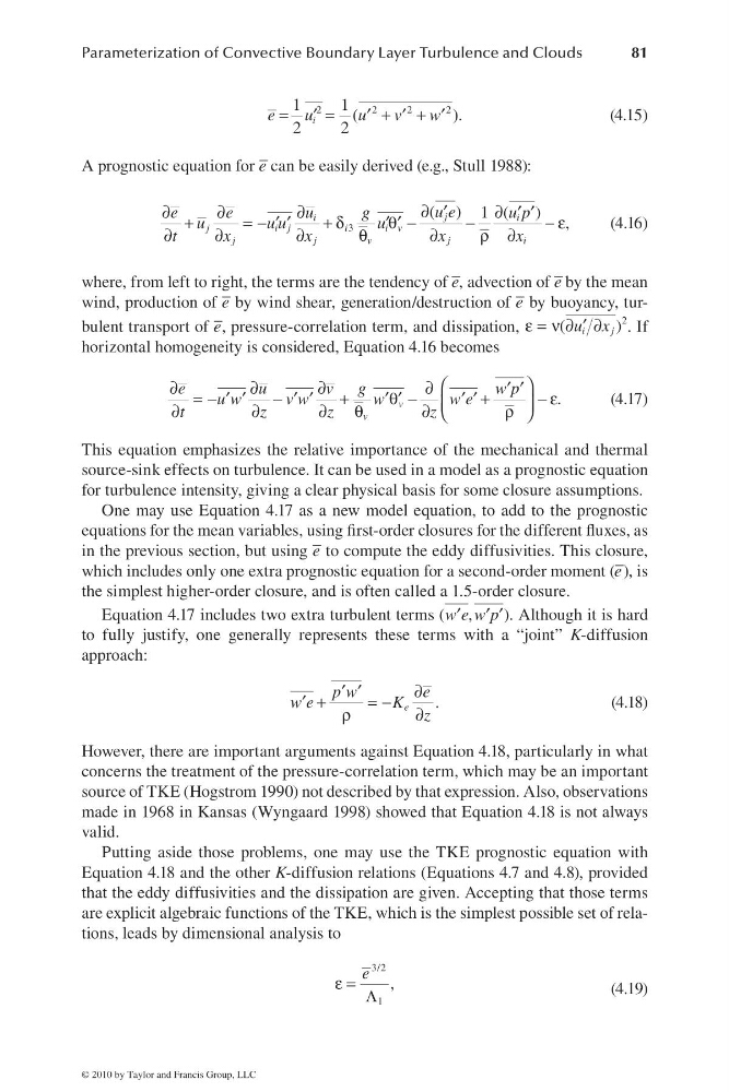
A prognostic equation for e – can be easily derived (e.g., Stull 1988):
3
( ) 1 (
) ,
j
i
i
j
ij
i
iv
j
j
v
j
i
u e
e
e
u
g
up
u
uu
u
t
x
x
x
x
∂ ′
∂
∂
∂
∂ ′ ′
+
=−
+δ
θ −
−
−ε
′ ′
′ ′
∂
∂
∂
θ
∂
ρ ∂
(4.16)
where, from left to right, the terms are the tendency of e – , advection of e – by the mean
wind, production of e – by wind shear, generation/destruction of e – by buoyancy, turbulent transport of e – , pressure-correlation term, and dissipation,
2
(
)
i
j
u x
ε = ν ∂ ∂
′
. If
horizontal homogeneity is considered, Equation 4.16 becomes
.
v
v
e
u
v g
wp
u w
v w
w
w e
t
z
z
z
⎛
⎞
∂
∂
∂
∂
′ ′
= −
−
+
θ −
+
− ε
′ ′
′ ′
′ ′
′ ′
⎜
⎟
∂
∂
∂
θ
∂
ρ
⎝
⎠
(4.17)
This equation emphasizes the relative importance of the mechanical and thermal
source-sink effects on turbulence. It can be used in a model as a prognostic equation
for turbulence intensity, giving a clear physical basis for some closure assumptions.
One may use Equation 4.17 as a new model equation, to add to the prognostic
equations for the mean variables, using fi rst-order closures for the different fl uxes, as
in the previous section, but using e – to compute the eddy diffusivities. This closure,
which includes only one extra prognostic equation for a second-order moment (e – ), is
the simplest higher-order closure, and is often called a 1.5-order closure.
Equation 4.17 includes two extra turbulent terms ( ,
)
w e w p
′ ′ ′ . Although it is hard
to fully justify, one generally represents these terms with a “joint” K-diffusion
approach:
∂
′ ′
+
=−
′
ρ
∂
.
e
p w
e
w e
K
z
(4.18)
However, there are important arguments against Equation 4.18, particularly in what
concerns the treatment of the pressure-correlation term, which may be an important
source of TKE (Hogstrom 1990) not described by that expression. Also, observations
made in 1968 in Kansas (Wyngaard 1998) showed that Equation 4.18 is not always
valid.
Putting aside those problems, one may use the TKE prognostic equation with
Equation 4.18 and the other K-diffusion relations (Equations 4.7 and 4.8), provided
that the eddy diffusivities and the dissipation are given. Accepting that those terms
are explicit algebraic functions of the TKE, which is the simplest possible set of relations, leads by dimensional analysis to
3/2
1
,
e
ε = Λ
(4.19)
© 2010 by Taylor and Francis Group, LLC
81
2
2
2
2
1
1 (
) .
2
2
i
e
u
u
v
w
=
=
+
+
′
′
′
′
(4.15)
A prognostic equation for e – can be easily derived (e.g., Stull 1988):
3
( ) 1 (
) ,
j
i
i
j
ij
i
iv
j
j
v
j
i
u e
e
e
u
g
up
u
uu
u
t
x
x
x
x
∂ ′
∂
∂
∂
∂ ′ ′
+
=−
+δ
θ −
−
−ε
′ ′
′ ′
∂
∂
∂
θ
∂
ρ ∂
(4.16)
where, from left to right, the terms are the tendency of e – , advection of e – by the mean
wind, production of e – by wind shear, generation/destruction of e – by buoyancy, turbulent transport of e – , pressure-correlation term, and dissipation,
2
(
)
i
j
u x
ε = ν ∂ ∂
′
. If
horizontal homogeneity is considered, Equation 4.16 becomes
.
v
v
e
u
v g
wp
u w
v w
w
w e
t
z
z
z
⎛
⎞
∂
∂
∂
∂
′ ′
= −
−
+
θ −
+
− ε
′ ′
′ ′
′ ′
′ ′
⎜
⎟
∂
∂
∂
θ
∂
ρ
⎝
⎠
(4.17)
This equation emphasizes the relative importance of the mechanical and thermal
source-sink effects on turbulence. It can be used in a model as a prognostic equation
for turbulence intensity, giving a clear physical basis for some closure assumptions.
One may use Equation 4.17 as a new model equation, to add to the prognostic
equations for the mean variables, using fi rst-order closures for the different fl uxes, as
in the previous section, but using e – to compute the eddy diffusivities. This closure,
which includes only one extra prognostic equation for a second-order moment (e – ), is
the simplest higher-order closure, and is often called a 1.5-order closure.
Equation 4.17 includes two extra turbulent terms ( ,
)
w e w p
′ ′ ′ . Although it is hard
to fully justify, one generally represents these terms with a “joint” K-diffusion
approach:
∂
′ ′
+
=−
′
ρ
∂
.
e
p w
e
w e
K
z
(4.18)
However, there are important arguments against Equation 4.18, particularly in what
concerns the treatment of the pressure-correlation term, which may be an important
source of TKE (Hogstrom 1990) not described by that expression. Also, observations
made in 1968 in Kansas (Wyngaard 1998) showed that Equation 4.18 is not always
valid.
Putting aside those problems, one may use the TKE prognostic equation with
Equation 4.18 and the other K-diffusion relations (Equations 4.7 and 4.8), provided
that the eddy diffusivities and the dissipation are given. Accepting that those terms
are explicit algebraic functions of the TKE, which is the simplest possible set of relations, leads by dimensional analysis to
3/2
1
,
e
ε = Λ
(4.19)
© 2010 by Taylor and Francis Group, LLC