

80
Air Pollution and Turbulence: Modeling and Applications
The technological advances in the measurement instruments of the turbulence
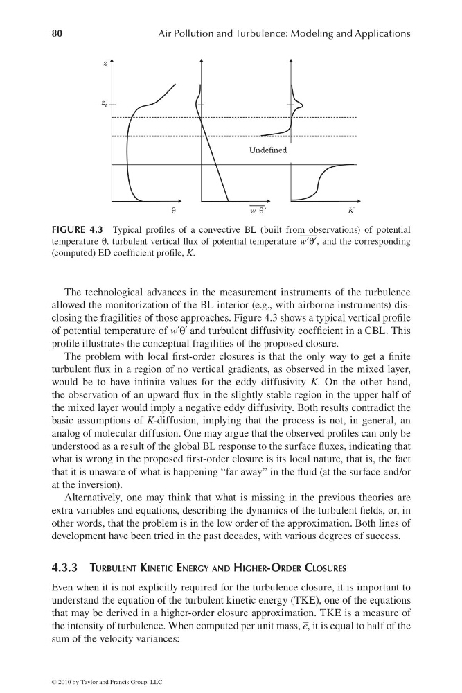
allowed the monitorization of the BL interior (e.g., with airborne instruments) disclosing the fragilities of those approaches. Figure 4.3 shows a typical vertical profi le
of potential temperature of w′ ′
θ and turbulent diffusivity coeffi cient in a CBL. This
profi le illustrates the conceptual fragilities of the proposed closure.
The problem with local fi rst-order closures is that the only way to get a fi nite
turbulent fl ux in a region of no vertical gradients, as observed in the mixed layer,
would be to have infi nite values for the eddy diffusivity K. On the other hand,
the observation of an upward fl ux in the slightly stable region in the upper half of
the mixed layer would imply a negative eddy diffusivity. Both results contradict the
basic assumptions of K-diffusion, implying that the process is not, in general, an
analog of molecular diffusion. One may argue that the observed profi les can only be
understood as a result of the global BL response to the surface fl uxes, indicating that
what is wrong in the proposed fi rst-order closure is its local nature, that is, the fact
that it is unaware of what is happening “far away” in the fl uid (at the surface and/or
at the inversion).
Alternatively, one may think that what is missing in the previous theories are
extra variables and equations, describing the dynamics of the turbulent fi elds, or, in
other words, that the problem is in the low order of the approximation. Both lines of
development have been tried in the past decades, with various degrees of success.
4.3.3 TURBULENT KINETIC ENERGY AND HIGHER-ORDER CLOSURES
Even when it is not explicitly required for the turbulence closure, it is important to
understand the equation of the turbulent kinetic energy (TKE), one of the equations
that may be derived in a higher-order closure approximation. TKE is a measure of
the intensity of turbulence. When computed per unit mass, e – , it is equal to half of the
sum of the velocity variances:
K
Undefined
z
z i
w΄θ΄
θ
FIGURE 4.3 Typical profi les of a convective BL (built from observations) of potential
temperature θ, turbulent vertical fl ux of potential temperature θ
′ ′
w , and the corresponding
( computed) ED coeffi cient profi le, K.
© 2010 by Taylor and Francis Group, LLC
Air Pollution and Turbulence: Modeling and Applications
The technological advances in the measurement instruments of the turbulence
allowed the monitorization of the BL interior (e.g., with airborne instruments) disclosing the fragilities of those approaches. Figure 4.3 shows a typical vertical profi le
of potential temperature of w′ ′
θ and turbulent diffusivity coeffi cient in a CBL. This
profi le illustrates the conceptual fragilities of the proposed closure.
The problem with local fi rst-order closures is that the only way to get a fi nite
turbulent fl ux in a region of no vertical gradients, as observed in the mixed layer,
would be to have infi nite values for the eddy diffusivity K. On the other hand,
the observation of an upward fl ux in the slightly stable region in the upper half of
the mixed layer would imply a negative eddy diffusivity. Both results contradict the
basic assumptions of K-diffusion, implying that the process is not, in general, an
analog of molecular diffusion. One may argue that the observed profi les can only be
understood as a result of the global BL response to the surface fl uxes, indicating that
what is wrong in the proposed fi rst-order closure is its local nature, that is, the fact
that it is unaware of what is happening “far away” in the fl uid (at the surface and/or
at the inversion).
Alternatively, one may think that what is missing in the previous theories are
extra variables and equations, describing the dynamics of the turbulent fi elds, or, in
other words, that the problem is in the low order of the approximation. Both lines of
development have been tried in the past decades, with various degrees of success.
4.3.3 TURBULENT KINETIC ENERGY AND HIGHER-ORDER CLOSURES
Even when it is not explicitly required for the turbulence closure, it is important to
understand the equation of the turbulent kinetic energy (TKE), one of the equations
that may be derived in a higher-order closure approximation. TKE is a measure of
the intensity of turbulence. When computed per unit mass, e – , it is equal to half of the
sum of the velocity variances:
K
Undefined
z
z i
w΄θ΄
θ
FIGURE 4.3 Typical profi les of a convective BL (built from observations) of potential
temperature θ, turbulent vertical fl ux of potential temperature θ
′ ′
w , and the corresponding
( computed) ED coeffi cient profi le, K.
© 2010 by Taylor and Francis Group, LLC