

Turbulence and Dispersion of Contaminants in the Planetary Boundary Layer 61
is considered. For large diffusion travel times, the eddy diffusivity has the form
(Hanna, 1981)
α
π β σ
=
α =
2 ( ; )
( ; )
,
, ,
3
( )
i
i
m i
t z
K t z
x y z
U k
(3.103)
where
(k m ) i is the wave number of the spectral peak (associated to the energy-containing
eddies)
U is the mean wind speed
β i is defi ned as the ratio of the Lagrangian to the Eulerian integral timescales
Considering β =
σ
0.55( / )
i
i
U
(Hanna, 1981; Degrazia et al., 1998) in Equation
3.103 yields the following decaying eddy diffusivity
α
π σ
=
0.55
( ; )
( ; )
3
( )
i
m i
t z
K t z
k
(3.104)
where, for our model, σ i (t;z) is obtained from Equations 3.96, 3.97, 3.99, 3.101, and 3.102.
Nieuwstadt and Brost (1986) report that the vertical velocity spectrum (depicted
in Figure 14 of their article), computed for several dimensionless times, all have a
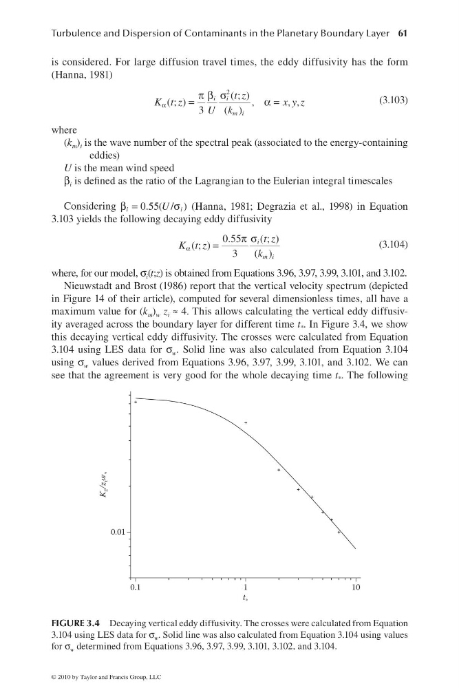
maximum value for (k m ) w z i ≈ 4. This allows calculating the vertical eddy diffusivity averaged across the boundary layer for different time t * . In Figure 3.4, we show
this decaying vertical eddy diffusivity. The crosses were calculated from Equation
3.104 using LES data for σ w . Solid line was also calculated from Equation 3.104
using σ w values derived from Equations 3.96, 3.97, 3.99, 3.101, and 3.102. We can
see that the agreement is very good for the whole decaying time t * . The following
K
z /z
i w
*
0.01
0.1
1
t *
10
FIGURE 3.4 Decaying vertical eddy diffusivity. The crosses were calculated from Equation
3.104 using LES data for σ w . Solid line was also calculated from Equation 3.104 using values
for σ w determined from Equations 3.96, 3.97, 3.99, 3.101, 3.102, and 3.104.
© 2010 by Taylor and Francis Group, LLC
is considered. For large diffusion travel times, the eddy diffusivity has the form
(Hanna, 1981)
α
π β σ
=
α =
2 ( ; )
( ; )
,
, ,
3
( )
i
i
m i
t z
K t z
x y z
U k
(3.103)
where
(k m ) i is the wave number of the spectral peak (associated to the energy-containing
eddies)
U is the mean wind speed
β i is defi ned as the ratio of the Lagrangian to the Eulerian integral timescales
Considering β =
σ
0.55( / )
i
i
U
(Hanna, 1981; Degrazia et al., 1998) in Equation
3.103 yields the following decaying eddy diffusivity
α
π σ
=
0.55
( ; )
( ; )
3
( )
i
m i
t z
K t z
k
(3.104)
where, for our model, σ i (t;z) is obtained from Equations 3.96, 3.97, 3.99, 3.101, and 3.102.
Nieuwstadt and Brost (1986) report that the vertical velocity spectrum (depicted
in Figure 14 of their article), computed for several dimensionless times, all have a
maximum value for (k m ) w z i ≈ 4. This allows calculating the vertical eddy diffusivity averaged across the boundary layer for different time t * . In Figure 3.4, we show
this decaying vertical eddy diffusivity. The crosses were calculated from Equation
3.104 using LES data for σ w . Solid line was also calculated from Equation 3.104
using σ w values derived from Equations 3.96, 3.97, 3.99, 3.101, and 3.102. We can
see that the agreement is very good for the whole decaying time t * . The following
K
z /z
i w
*
0.01
0.1
1
t *
10
FIGURE 3.4 Decaying vertical eddy diffusivity. The crosses were calculated from Equation
3.104 using LES data for σ w . Solid line was also calculated from Equation 3.104 using values
for σ w determined from Equations 3.96, 3.97, 3.99, 3.101, 3.102, and 3.104.
© 2010 by Taylor and Francis Group, LLC