Turbulence and Dispersion of Contaminants in the Planetary Boundary Layer 49
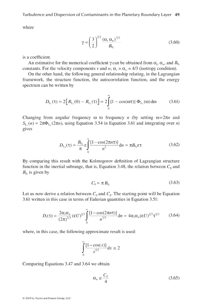
where
α α
⎛ ⎞
γ = ⎜ ⎟
⎝ ⎠
3 2
3 2
0
3
(
)
2
i
i u
B
(3.60)
is a coeffi cient.
An estimative for the numerical coeffi cient γ can be obtained from α i , α u , and 0 i
B
constants. For the velocity components v and w, α v = α w = 4/3 (isotropy condition).
On the other hand, the following general relationship relating, in the Lagrangian
framework, the structure function, the autocorrelation function, and the energy
spectrum can be written by
∞
τ =
−
τ =
−
ωτ Φ ω ω
⎡
⎤
⎣
⎦
∫
L
L
L
L
0
( ) 2
(0)
( )
2 [1 cos( )]
( )d
i
i
i
i
D
R
R
(3.61)
Changing from angular frequency ω to frequency n (by setting ω = 2πn and
= πΦ
π
L
L
( ) 2
(2 )
i
i
S n
n , using Equation 3.54 in Equation 3.61 and integrating over n)
gives
∞
−
π τ
τ =
ε
= π ετ
π ∫
i
0
L
0
2
0
[1 cos(2
)]
( )
d
i
i
B
n
D
n
B
n
(3.62)
By comparing this result with the Kolmogorov defi nition of Lagrangian structure
function in the inertial subrange, that is, Equation 3.48, the relation between C 0 and
0 i
B is given by
= π
0
0 i
C
B
(3.63)
Let us now derive a relation between C 0 and C S . The starting point will be Equation
3.61 written in this case in terms of Eulerian quantities in Equation 3.51:
∞
α α
−
π τ
τ =
ε
≈ α α ε
τ
π
∫
2 3
2 3 2 3
2 3
2 3
0
2
[ 1 c o s ( 2
) ]
( )
( )
d
4
( )
(2 )
i u
i
i u
n
D
U
n
U
n
(3.64)
where, in this case, the following approximate result is used:
∞
−
≅
∫ 5 3
0
[1 cos( )] d
2
x x
x
Comparing Equations 3.47 and 3.64 we obtain
4
S
u
C
α ≅
(3.65)
© 2010 by Taylor and Francis Group, LLC