

292
Air Pollution and Turbulence: Modeling and Applications
However, one of the most important characteristics of synthesis inversion is that
the fi t can be, and since 1995 usually is, performed as a statistical fi t and weighted to
take into account the uncertainties in the data. Using the generic notation of Section
11.2.2 (as opposed to the specifi c discretization of (Equation 11.4a through 11.4d)),
with z as a data vector, x as a generic discretization of fl uxes, and G as the corresponding Green’s functions (
[ ]
k
c
α ), leads to the cost functions 11.4a or 11.4b. In the
absence of a Bayesian constraint, Equation 11.4a must be supplemented by some
other form of regularization.
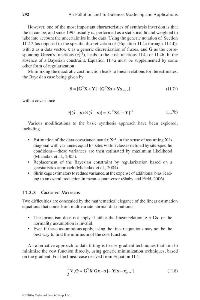
Minimizing the quadratic cost function leads to linear relations for the estimates,
the Bayesian case being given by
T
1
T
prior
ˆ [
] [
]
−
=
+
+
x G X Y G Xz Yx
(11.7a)
with a covariance
T
1
ˆ
ˆ
E[(
) (
)] [
]
−
− ⊗ −
=
+
x x
x x
G XG Y
(11.7b)
Various modifi cations to the basic synthesis approach have been explored,
including
Estimation of the data covariance matrix
•
X −1 , in the sense of assuming X is
diagonal with variances equal for sites within classes defi ned by site-specifi c
conditions—these variances are then estimated by maximum likelihood
(Michalak et al., 2005).
Replacement of the Bayesian constraint by regularization based on a
•
geostatistics approach (Michalak et al., 2004).
Shrinkage estimators to reduce variance, at the expense of additional bias, lead•
ing to an overall reduction in mean-square-error (Shaby and Field, 2006).
11.2.3 GRADIENT METHODS
Two diffi culties are concealed by the mathematical elegance of the linear estimation
equations that come from multivariate normal distributions:
The formalism does not apply if either the linear relation,
•
z ≈ Gx, or the
normality assumption is invalid.
Even if these assumptions apply, using the linear equations may not be the
•
best way to fi nd the minimum of the cost function.
An alternative approach to data fi tting is to use gradient techniques that aim to
minimize the cost function directly, using generic minimization techniques, based
on the gradient. For the linear case derived from Equation 11.4:
∇ Θ =
− +
−
x
p r i o r
1
[
]
[
]
2
T
G X Gx z Y x x
(11.8)
© 2010 by Taylor and Francis Group, LLC
Air Pollution and Turbulence: Modeling and Applications
However, one of the most important characteristics of synthesis inversion is that
the fi t can be, and since 1995 usually is, performed as a statistical fi t and weighted to
take into account the uncertainties in the data. Using the generic notation of Section
11.2.2 (as opposed to the specifi c discretization of (Equation 11.4a through 11.4d)),
with z as a data vector, x as a generic discretization of fl uxes, and G as the corresponding Green’s functions (
[ ]
k
c
α ), leads to the cost functions 11.4a or 11.4b. In the
absence of a Bayesian constraint, Equation 11.4a must be supplemented by some
other form of regularization.
Minimizing the quadratic cost function leads to linear relations for the estimates,
the Bayesian case being given by
T
1
T
prior
ˆ [
] [
]
−
=
+
+
x G X Y G Xz Yx
(11.7a)
with a covariance
T
1
ˆ
ˆ
E[(
) (
)] [
]
−
− ⊗ −
=
+
x x
x x
G XG Y
(11.7b)
Various modifi cations to the basic synthesis approach have been explored,
including
Estimation of the data covariance matrix
•
X −1 , in the sense of assuming X is
diagonal with variances equal for sites within classes defi ned by site-specifi c
conditions—these variances are then estimated by maximum likelihood
(Michalak et al., 2005).
Replacement of the Bayesian constraint by regularization based on a
•
geostatistics approach (Michalak et al., 2004).
Shrinkage estimators to reduce variance, at the expense of additional bias, lead•
ing to an overall reduction in mean-square-error (Shaby and Field, 2006).
11.2.3 GRADIENT METHODS
Two diffi culties are concealed by the mathematical elegance of the linear estimation
equations that come from multivariate normal distributions:
The formalism does not apply if either the linear relation,
•
z ≈ Gx, or the
normality assumption is invalid.
Even if these assumptions apply, using the linear equations may not be the
•
best way to fi nd the minimum of the cost function.
An alternative approach to data fi tting is to use gradient techniques that aim to
minimize the cost function directly, using generic minimization techniques, based
on the gradient. For the linear case derived from Equation 11.4:
∇ Θ =
− +
−
x
p r i o r
1
[
]
[
]
2
T
G X Gx z Y x x
(11.8)
© 2010 by Taylor and Francis Group, LLC