

Inversion of Atmospheric CO 2 Concentrations
291
This means that at all the surface sites, one needs to know the c j (t) and their rates
of change. Given the tendency of numerical differentiation to amplify noise, this
requires smoothing of the data.
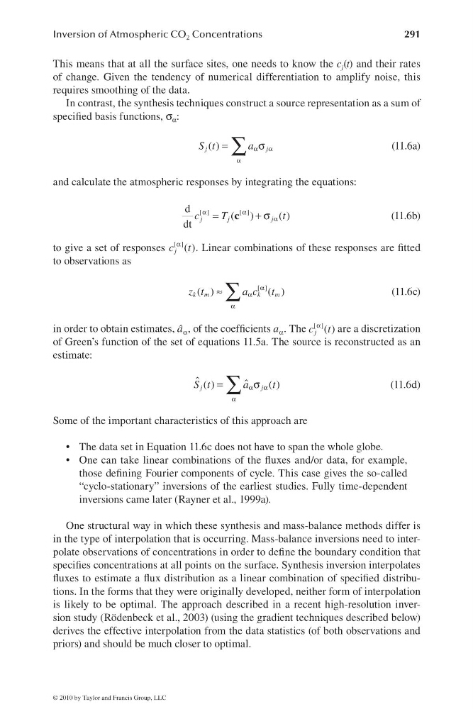
In contrast, the synthesis techniques construct a source representation as a sum of
specifi ed basis functions, σ α :
( )
j
j
S t
a α α
α
=
σ
∑
(11.6a)
and calculate the atmospheric responses by integrating the equations:
[ ]
[ ]
d
( )
( )
dt
j
j
j
c
T
t
α
α
α
=
+σ
c
(11.6b)
to give a set of responses
[ ] ( )
j
c t
α
. Linear combinations of these responses are fi tted
to observations as
[ ]
( )
( )
k m
k
m
z t
a c t
α
α
α
≈ ∑
(11.6c)
in order to obtain estimates, â α , of the coeffi cients a α . The
[ ] ( )
j
c t
α
are a discretization
of Green’s function of the set of equations 11.5a. The source is reconstructed as an
estimate:
ˆ
ˆ
( )
( )
j
j
S t
a
t
α
α
α
=
σ
∑
(11.6d)
Some of the important characteristics of this approach are
The data set in Equation 11.6c does not have to span the whole globe.
•
One can take linear combinations of the fl uxes and/or data, for example,
•
those defi ning Fourier components of cycle. This case gives the so-called
“cyclo-stationary” inversions of the earliest studies. Fully time-dependent
inversions came later (Rayner et al., 1999a).
One structural way in which these synthesis and mass-balance methods differ is
in the type of interpolation that is occurring. Mass-balance inversions need to interpolate observations of concentrations in order to defi ne the boundary condition that
specifi es concentrations at all points on the surface. Synthesis inversion interpolates
fl uxes to estimate a fl ux distribution as a linear combination of specifi ed distributions. In the forms that they were originally developed, neither form of interpolation
is likely to be optimal. The approach described in a recent high-resolution inversion study (Rödenbeck et al., 2003) (using the gradient techniques described below)
derives the effective interpolation from the data statistics (of both observations and
priors) and should be much closer to optimal.
© 2010 by Taylor and Francis Group, LLC
291
This means that at all the surface sites, one needs to know the c j (t) and their rates
of change. Given the tendency of numerical differentiation to amplify noise, this
requires smoothing of the data.
In contrast, the synthesis techniques construct a source representation as a sum of
specifi ed basis functions, σ α :
( )
j
j
S t
a α α
α
=
σ
∑
(11.6a)
and calculate the atmospheric responses by integrating the equations:
[ ]
[ ]
d
( )
( )
dt
j
j
j
c
T
t
α
α
α
=
+σ
c
(11.6b)
to give a set of responses
[ ] ( )
j
c t
α
. Linear combinations of these responses are fi tted
to observations as
[ ]
( )
( )
k m
k
m
z t
a c t
α
α
α
≈ ∑
(11.6c)
in order to obtain estimates, â α , of the coeffi cients a α . The
[ ] ( )
j
c t
α
are a discretization
of Green’s function of the set of equations 11.5a. The source is reconstructed as an
estimate:
ˆ
ˆ
( )
( )
j
j
S t
a
t
α
α
α
=
σ
∑
(11.6d)
Some of the important characteristics of this approach are
The data set in Equation 11.6c does not have to span the whole globe.
•
One can take linear combinations of the fl uxes and/or data, for example,
•
those defi ning Fourier components of cycle. This case gives the so-called
“cyclo-stationary” inversions of the earliest studies. Fully time-dependent
inversions came later (Rayner et al., 1999a).
One structural way in which these synthesis and mass-balance methods differ is
in the type of interpolation that is occurring. Mass-balance inversions need to interpolate observations of concentrations in order to defi ne the boundary condition that
specifi es concentrations at all points on the surface. Synthesis inversion interpolates
fl uxes to estimate a fl ux distribution as a linear combination of specifi ed distributions. In the forms that they were originally developed, neither form of interpolation
is likely to be optimal. The approach described in a recent high-resolution inversion study (Rödenbeck et al., 2003) (using the gradient techniques described below)
derives the effective interpolation from the data statistics (of both observations and
priors) and should be much closer to optimal.
© 2010 by Taylor and Francis Group, LLC