

262
Air Pollution and Turbulence: Modeling and Applications
with a (mean) growth rate λ known as the maximum Lyapunov exponent (MLE).
The Lagrangian description of fl uid motion can also be seen from a dynamical systems point of view. In fact, in the Lagrangian framework, the vector x
→ is the tracer
trajectory, the operator F
→
is the velocity fi eld, and the error δx
→ is the distance between
two tracer trajectories. It is therefore straightforward to consider the relative dispersion of Lagrangian trajectories as a problem of fi nite-error predictability.
The importance of the fi nite-scale analysis will become clear as this tool permits us to overcome the diffi culties noted in the last section and that usually appear
when trying to study the relative dispersion in fully developed turbulence (i.e., high
Reynolds numbers turbulence) by means of the time-dependent approach. However,
in many recent works, the FSLE analysis has been used as diagnostic of transport
properties in geophysical systems (e.g., Lacorata et al., 2001). Before introducing the
fi nite size analysis for dispersion problems, we recall what asymptotic regimes hold
for N particle pairs advected by a Eulerian velocity fi eld u
→ (x
→
,t) characterized by two
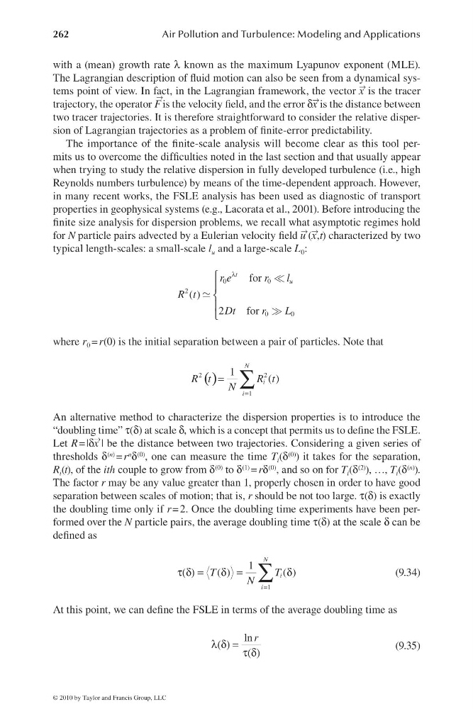
typical length-scales: a small-scale l u and a large-scale L 0 :
λ
⎧
⎪
⎨
⎪
⎩
0
0
2
0
0
for
( )
2
for
t
u
r e
r
l
R t
Dt
r
L
where r 0 = r(0) is the initial separation between a pair of particles. Note that
( )
=
= ∑
2
2
1
1
( )
N
i
i
R t
R t
N
An alternative method to characterize the dispersion properties is to introduce the
“doubling time” τ(δ) at scale δ, which is a concept that permits us to defi ne the FSLE.
Let R = |δx
→ | be the distance between two trajectories. Considering a given series of
thresholds δ (n) = r n δ (0) , one can measure the time T i (δ (0) ) it takes for the separation,
R i (t), of the ith couple to grow from δ (0) to δ (1) = rδ (0) , and so on for T i (δ (2) ), …, T i (δ (n) ).
The factor r may be any value greater than 1, properly chosen in order to have good
separation between scales of motion; that is, r should be not too large. τ(δ) is exactly
the doubling time only if r = 2. Once the doubling time experiments have been performed over the N particle pairs, the average doubling time τ(δ) at the scale δ can be
defi ned as
1
1
( )
( )
N
i
i
T
T
N =
τ(δ) =
δ =
δ
∑
(9.34)
At this point, we can defi ne the FSLE in terms of the average doubling time as
ln r
λ(δ) = τ(δ)
(9.35)
© 2010 by Taylor and Francis Group, LLC
Air Pollution and Turbulence: Modeling and Applications
with a (mean) growth rate λ known as the maximum Lyapunov exponent (MLE).
The Lagrangian description of fl uid motion can also be seen from a dynamical systems point of view. In fact, in the Lagrangian framework, the vector x
→ is the tracer
trajectory, the operator F
→
is the velocity fi eld, and the error δx
→ is the distance between
two tracer trajectories. It is therefore straightforward to consider the relative dispersion of Lagrangian trajectories as a problem of fi nite-error predictability.
The importance of the fi nite-scale analysis will become clear as this tool permits us to overcome the diffi culties noted in the last section and that usually appear
when trying to study the relative dispersion in fully developed turbulence (i.e., high
Reynolds numbers turbulence) by means of the time-dependent approach. However,
in many recent works, the FSLE analysis has been used as diagnostic of transport
properties in geophysical systems (e.g., Lacorata et al., 2001). Before introducing the
fi nite size analysis for dispersion problems, we recall what asymptotic regimes hold
for N particle pairs advected by a Eulerian velocity fi eld u
→ (x
→
,t) characterized by two
typical length-scales: a small-scale l u and a large-scale L 0 :
λ
⎧
⎪
⎨
⎪
⎩
0
0
2
0
0
for
( )
2
for
t
u
r e
r
l
R t
Dt
r
L
where r 0 = r(0) is the initial separation between a pair of particles. Note that
( )
=
= ∑
2
2
1
1
( )
N
i
i
R t
R t
N
An alternative method to characterize the dispersion properties is to introduce the
“doubling time” τ(δ) at scale δ, which is a concept that permits us to defi ne the FSLE.
Let R = |δx
→ | be the distance between two trajectories. Considering a given series of
thresholds δ (n) = r n δ (0) , one can measure the time T i (δ (0) ) it takes for the separation,
R i (t), of the ith couple to grow from δ (0) to δ (1) = rδ (0) , and so on for T i (δ (2) ), …, T i (δ (n) ).
The factor r may be any value greater than 1, properly chosen in order to have good
separation between scales of motion; that is, r should be not too large. τ(δ) is exactly
the doubling time only if r = 2. Once the doubling time experiments have been performed over the N particle pairs, the average doubling time τ(δ) at the scale δ can be
defi ned as
1
1
( )
( )
N
i
i
T
T
N =
τ(δ) =
δ =
δ
∑
(9.34)
At this point, we can defi ne the FSLE in terms of the average doubling time as
ln r
λ(δ) = τ(δ)
(9.35)
© 2010 by Taylor and Francis Group, LLC