

Atmospheric Dispersion with a Large-Eddy Simulation
239
As a consequence, a direct numerical simulation (DNS), where all turbulent fl ow
scales are solved numerically, is a simulation, while a large-eddy simulation (LES)
is a compromise between simulation and modeling. In fact, in an LES, only the
energy-containing eddies (ECE) are simulated, while the rest are modeled. The
proper distinction between fl ow scales is accomplished by applying a high-pass fi lter, with a cut-off length Δ f , to the Navier–Stokes equations. It is clear that LES will
provide satisfactory results when the cut-off length Δ f is much smaller than the scale
of the ECE of the turbulence.
LES was used fi rst in micrometeorology by Deardorff (1970, 1972). The growth in
size, speed, and availability of supercomputers has since made LES more and more
suitable to PBL applications. The velocity and turbulence fi elds provided by LES can
be used to calculate the transport and dispersion of contaminants. In this way, one can
obtain, at the same time, detailed dispersion data and complete information on meteorological and turbulent parameters. Several studies with LES for atmospheric dispersion
have been reported in the literature and concern both Eulerian and Lagrangian dispersion simulation approaches (Nieuwstadt and De Valk, 1987; Van Haren and Nieuwstadt,
1989; Kemp and Thompson, 1996; Meeder and Nieuwstadt, 2000; Rizza et al., 2006).
We assume that the theoretical background and the principal differences between
the most important instruments in computational fl uid dynamics (CFD), that is, DNS,
LES, and RANS (Reynolds averaged Navier–Stokes) are known, so we describe very
briefl y Moeng’s LES code used in the present work.
Both approaches for studying turbulent dispersion, the Eulerian and the Lagrangian
frameworks, are used by means of LESs. In fact, both of these approaches have peculiar
aspects that we must examine. Lagrangian particle models can successfully describe
the turbulent dispersion of passive contaminants because they take into account essential aspects of turbulence, but they are limited to a simplifi ed set of reacting species.
The Eulerian approach, on the other hand, is based on the conservation equation and
can incorporate the numerous second and high-order chemical kinetic equations necessary to describe photochemical smog generation, which currently represents a challenging environmental problem. The critical point is the numerical scheme used to
discretize the conservation equation, which can generate nonphysical results.
9.2 LARGE-EDDY SIMULATION: THE MOENG
AND SULLIVAN MODEL
9.2.1 DESCRIPTION
The large-eddy model used in this study is the LES model developed by Moeng
(1984) and Sullivan et al. (1994). Here, we only give a short outcome.
In the LES technique, the smallest eddies in a large Reynolds number PBL fl ow
are removed by applying a spatial fi lter function to the Navier–Stokes equations. For
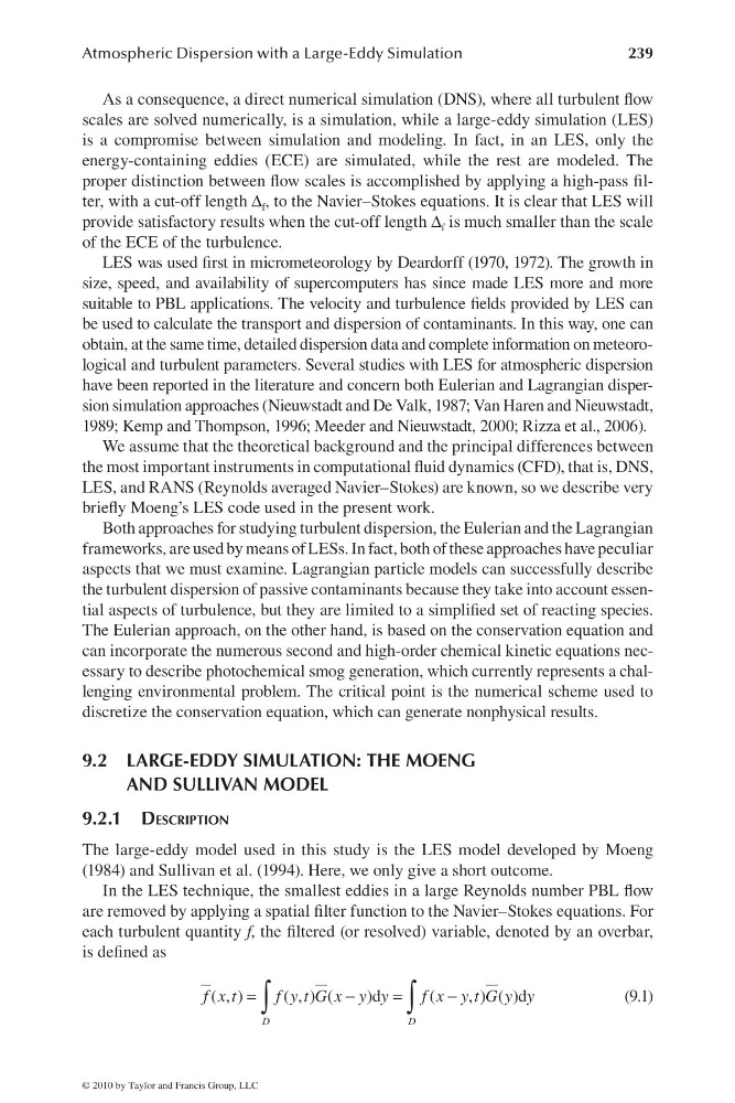
each turbulent quantity f, the fi ltered (or resolved) variable, denoted by an overbar,
is defi ned as
=
−
=
−
∫
∫
( , )
( , ) (
)d
(
, ) ( )d
D
D
f x t
f y t G x y y
f x y t G y y
(9.1)
© 2010 by Taylor and Francis Group, LLC
239
As a consequence, a direct numerical simulation (DNS), where all turbulent fl ow
scales are solved numerically, is a simulation, while a large-eddy simulation (LES)
is a compromise between simulation and modeling. In fact, in an LES, only the
energy-containing eddies (ECE) are simulated, while the rest are modeled. The
proper distinction between fl ow scales is accomplished by applying a high-pass fi lter, with a cut-off length Δ f , to the Navier–Stokes equations. It is clear that LES will
provide satisfactory results when the cut-off length Δ f is much smaller than the scale
of the ECE of the turbulence.
LES was used fi rst in micrometeorology by Deardorff (1970, 1972). The growth in
size, speed, and availability of supercomputers has since made LES more and more
suitable to PBL applications. The velocity and turbulence fi elds provided by LES can
be used to calculate the transport and dispersion of contaminants. In this way, one can
obtain, at the same time, detailed dispersion data and complete information on meteorological and turbulent parameters. Several studies with LES for atmospheric dispersion
have been reported in the literature and concern both Eulerian and Lagrangian dispersion simulation approaches (Nieuwstadt and De Valk, 1987; Van Haren and Nieuwstadt,
1989; Kemp and Thompson, 1996; Meeder and Nieuwstadt, 2000; Rizza et al., 2006).
We assume that the theoretical background and the principal differences between
the most important instruments in computational fl uid dynamics (CFD), that is, DNS,
LES, and RANS (Reynolds averaged Navier–Stokes) are known, so we describe very
briefl y Moeng’s LES code used in the present work.
Both approaches for studying turbulent dispersion, the Eulerian and the Lagrangian
frameworks, are used by means of LESs. In fact, both of these approaches have peculiar
aspects that we must examine. Lagrangian particle models can successfully describe
the turbulent dispersion of passive contaminants because they take into account essential aspects of turbulence, but they are limited to a simplifi ed set of reacting species.
The Eulerian approach, on the other hand, is based on the conservation equation and
can incorporate the numerous second and high-order chemical kinetic equations necessary to describe photochemical smog generation, which currently represents a challenging environmental problem. The critical point is the numerical scheme used to
discretize the conservation equation, which can generate nonphysical results.
9.2 LARGE-EDDY SIMULATION: THE MOENG
AND SULLIVAN MODEL
9.2.1 DESCRIPTION
The large-eddy model used in this study is the LES model developed by Moeng
(1984) and Sullivan et al. (1994). Here, we only give a short outcome.
In the LES technique, the smallest eddies in a large Reynolds number PBL fl ow
are removed by applying a spatial fi lter function to the Navier–Stokes equations. For
each turbulent quantity f, the fi ltered (or resolved) variable, denoted by an overbar,
is defi ned as
=
−
=
−
∫
∫
( , )
( , ) (
)d
(
, ) ( )d
D
D
f x t
f y t G x y y
f x y t G y y
(9.1)
© 2010 by Taylor and Francis Group, LLC