

An Outline of Lagrangian Stochastic Dispersion Models
217
is a regression curve. They concluded that both methods satisfy the well-mixed
condition and do not appreciably depart from the exact solution. The second solution
is preferred for practical use since it is less time consuming.
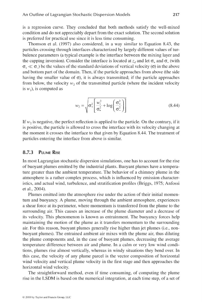
Thomson et al. (1997) also considered, in a way similar to Equation 8.43, the
particles crossing through interfaces characterized by largely different values of turbulence parameters (a typical example is the interface between the mixing layer and
the capping inversion). Consider the interface is located at z d and let σ + and σ − (with
σ + σ − ) be the values of the standard deviations of vertical velocity (σ) in the above
and bottom part of the domain. Then, if the particle approaches from above (the side
having the smaller value of σ), it is always transmitted; if the particle approaches
from below, the velocity w 2 of the transmitted particle (where the incident velocity
is w 1 ), is computed as
2
2
1
2
2
2
2
log
w
w
+
+
+
−
⎡
⎤
⎛ ⎞
σ
= σ
+
⎢
⎥
⎜ ⎟
σ
σ
⎝ ⎠
⎢
⎥
⎣
⎦
(8.44)
If w 2 is negative, the perfect refl ection is applied to the particle. On the contrary, if it
is positive, the particle is allowed to cross the interface with its velocity changing at
the moment it crosses the interface to that given by Equation 8.44. The treatment of
particles entering the interface from above is similar.
8.7.3 PLUME RISE
In most Lagrangian stochastic dispersion simulations, one has to account for the rise
of buoyant plumes emitted by the industrial plants. Buoyant plumes have a temperature greater than the ambient temperature. The behavior of a chimney plume in the
atmosphere is a rather complex process, which is infl uenced by emission characteristics, and actual wind, turbulence, and stratifi cation profi les (Briggs, 1975; Anfossi
et al., 2004).
Plumes emitted into the atmosphere rise under the action of their initial momentum and buoyancy. A plume, moving through the ambient atmosphere, experiences
a shear force at its perimeter, where momentum is transferred from the plume to the
surrounding air. This causes an increase of the plume diameter and a decrease of
its velocity. This phenomenon is known as entrainment. The buoyancy forces help
maintaining the motion of the plume as it transfers momentum to the surrounding
air. For this reason, buoyant plumes generally rise higher than jet plumes (i.e., nonbuoyant plumes). The entrained ambient air mixes with the plume air, thus diluting
the plume components and, in the case of buoyant plumes, decreasing the average
temperature difference between air and plume. In a calm or very low wind conditions, plumes rise almost vertically, whereas in windy situations they bend over. In
this case, the velocity of any plume parcel is the vector composition of horizontal
wind velocity and vertical plume velocity in the fi rst stage and then approaches the
horizontal wind velocity.
The straightforward method, even if time consuming, of computing the plume
rise in the LSDM is based on the numerical integration, at each time step, of a set of
© 2010 by Taylor and Francis Group, LLC
217
is a regression curve. They concluded that both methods satisfy the well-mixed
condition and do not appreciably depart from the exact solution. The second solution
is preferred for practical use since it is less time consuming.
Thomson et al. (1997) also considered, in a way similar to Equation 8.43, the
particles crossing through interfaces characterized by largely different values of turbulence parameters (a typical example is the interface between the mixing layer and
the capping inversion). Consider the interface is located at z d and let σ + and σ − (with
σ + σ − ) be the values of the standard deviations of vertical velocity (σ) in the above
and bottom part of the domain. Then, if the particle approaches from above (the side
having the smaller value of σ), it is always transmitted; if the particle approaches
from below, the velocity w 2 of the transmitted particle (where the incident velocity
is w 1 ), is computed as
2
2
1
2
2
2
2
log
w
w
+
+
+
−
⎡
⎤
⎛ ⎞
σ
= σ
+
⎢
⎥
⎜ ⎟
σ
σ
⎝ ⎠
⎢
⎥
⎣
⎦
(8.44)
If w 2 is negative, the perfect refl ection is applied to the particle. On the contrary, if it
is positive, the particle is allowed to cross the interface with its velocity changing at
the moment it crosses the interface to that given by Equation 8.44. The treatment of
particles entering the interface from above is similar.
8.7.3 PLUME RISE
In most Lagrangian stochastic dispersion simulations, one has to account for the rise
of buoyant plumes emitted by the industrial plants. Buoyant plumes have a temperature greater than the ambient temperature. The behavior of a chimney plume in the
atmosphere is a rather complex process, which is infl uenced by emission characteristics, and actual wind, turbulence, and stratifi cation profi les (Briggs, 1975; Anfossi
et al., 2004).
Plumes emitted into the atmosphere rise under the action of their initial momentum and buoyancy. A plume, moving through the ambient atmosphere, experiences
a shear force at its perimeter, where momentum is transferred from the plume to the
surrounding air. This causes an increase of the plume diameter and a decrease of
its velocity. This phenomenon is known as entrainment. The buoyancy forces help
maintaining the motion of the plume as it transfers momentum to the surrounding
air. For this reason, buoyant plumes generally rise higher than jet plumes (i.e., nonbuoyant plumes). The entrained ambient air mixes with the plume air, thus diluting
the plume components and, in the case of buoyant plumes, decreasing the average
temperature difference between air and plume. In a calm or very low wind conditions, plumes rise almost vertically, whereas in windy situations they bend over. In
this case, the velocity of any plume parcel is the vector composition of horizontal
wind velocity and vertical plume velocity in the fi rst stage and then approaches the
horizontal wind velocity.
The straightforward method, even if time consuming, of computing the plume
rise in the LSDM is based on the numerical integration, at each time step, of a set of
© 2010 by Taylor and Francis Group, LLC