

An Outline of Lagrangian Stochastic Dispersion Models
211
The use of this PDF in the Lagrangian stochastic models was proposed by
Anfossi et al. (1996) and Ferrero and Anfossi (1998a,b). Setting C 4 = 0 in Equation
8.26, one obtains the Gram-Charlier PDF truncated to third order (GC3), whereas
by setting C 3 = 0 as well, Equation 8.26 reduces to the Gaussian PDF. Gram-Charlier
series expansions, though showing good correspondence to experiments (see, for
instance, Frenkiel and Klebanoff, 1967; Durst et al., 1992; Anfossi et al., 1996), can
exhibit small negative probabilities in the tails of the distribution. However, numerical experiments (Ferrero and Anfossi, 1998b) found that these unrealistic velocities rarely occur and thus showed that discarding these nonphysical probabilities is
inconsequential in practical applications. On the other hand, the main advantages
of the Gram-Charlier PDFs are their computational effi ciency and their ability to
include information on the Eulerian moments directly.
8.4 SOLUTIONS OF THE 1-D LANGEVIN EQUATION
As above anticipated, in many applications concerning dispersion estimate in
convective conditions (in which the vertical turbulence is nonhomogeneous and
asymmetric) and fl at terrain, only the vertical velocity is computed by the Langevin
equation; thus a 1-D model is considered.
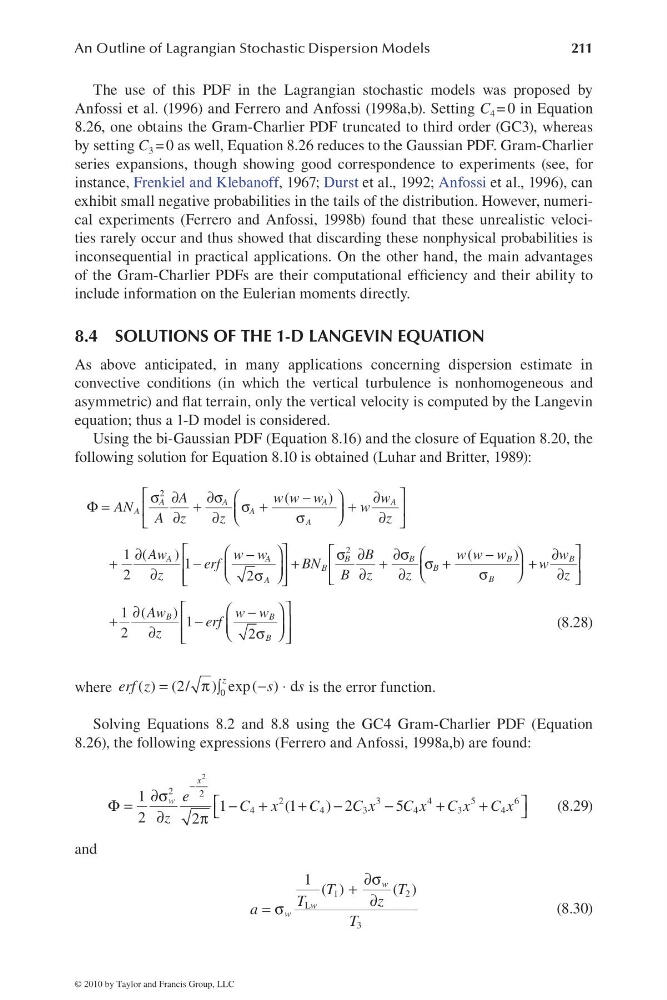
Using the bi-Gaussian PDF (Equation 8.16) and the closure of Equation 8.20, the
following solution for Equation 8.10 is obtained (Luhar and Britter, 1989):
⎡
⎤
⎛
⎞
σ ∂
∂σ
−
∂
Φ =
+
σ +
+
⎢
⎥
⎜
⎟
⎝
⎠
∂
∂
σ
∂
⎣
⎦
⎡
⎤
⎡
⎤
⎛
⎞
⎛
⎞
∂
−
σ∂
∂ σ
−
∂
+
−
+
+
σ+
+
⎢
⎥
⎢
⎥
⎜
⎟
⎜
⎟
⎝
⎠
∂
∂
∂
σ
∂
⎝
⎠
σ
⎢
⎥
⎣
⎦
⎣
⎦
⎡
⎤
⎛
⎞
∂
−
+
−
⎢
⎥
⎜
⎟
∂
⎝
⎠
σ
⎢
⎥
⎣
⎦
2
2
(
)
1 (
)
(
)
1
2
2
1 (
) 1
2
2
A
A
A
A
A
A
A
A
A
B
B
B
B
B
B
B
A
B
B
B
A
ww w
w
AN
w
A z
z
z
Aw
w w
B
w w w
w
erf
BN
w
z
Bz
z
z
Aw
w w
erf
z
(8.28)
where
=
π
− ⋅
∫ 0
( ) (2/ ) exp( ) d
z
erf z
s
s is the error function.
Solving Equations 8.2 and 8.8 using the GC4 Gram-Charlier PDF (Equation
8.26), the following expressions (Ferrero and Anfossi, 1998a,b) are found:
2
2
2
2
3
4
5
6
4
4
3
4
3
4
1
1
( 1
) 2
5
2
2
x
w e
C x
C
C x
C x C x C x
z
−
∂σ
⎡
⎤
Φ =
− +
+
−
−
+
+
⎣
⎦
∂
π
(8.29)
and
1
2
L
3
1 ( )
( )
w
w
w
T
T
T
z
a
T
∂σ
+ ∂
= σ
(8.30)
© 2010 by Taylor and Francis Group, LLC
211
The use of this PDF in the Lagrangian stochastic models was proposed by
Anfossi et al. (1996) and Ferrero and Anfossi (1998a,b). Setting C 4 = 0 in Equation
8.26, one obtains the Gram-Charlier PDF truncated to third order (GC3), whereas
by setting C 3 = 0 as well, Equation 8.26 reduces to the Gaussian PDF. Gram-Charlier
series expansions, though showing good correspondence to experiments (see, for
instance, Frenkiel and Klebanoff, 1967; Durst et al., 1992; Anfossi et al., 1996), can
exhibit small negative probabilities in the tails of the distribution. However, numerical experiments (Ferrero and Anfossi, 1998b) found that these unrealistic velocities rarely occur and thus showed that discarding these nonphysical probabilities is
inconsequential in practical applications. On the other hand, the main advantages
of the Gram-Charlier PDFs are their computational effi ciency and their ability to
include information on the Eulerian moments directly.
8.4 SOLUTIONS OF THE 1-D LANGEVIN EQUATION
As above anticipated, in many applications concerning dispersion estimate in
convective conditions (in which the vertical turbulence is nonhomogeneous and
asymmetric) and fl at terrain, only the vertical velocity is computed by the Langevin
equation; thus a 1-D model is considered.
Using the bi-Gaussian PDF (Equation 8.16) and the closure of Equation 8.20, the
following solution for Equation 8.10 is obtained (Luhar and Britter, 1989):
⎡
⎤
⎛
⎞
σ ∂
∂σ
−
∂
Φ =
+
σ +
+
⎢
⎥
⎜
⎟
⎝
⎠
∂
∂
σ
∂
⎣
⎦
⎡
⎤
⎡
⎤
⎛
⎞
⎛
⎞
∂
−
σ∂
∂ σ
−
∂
+
−
+
+
σ+
+
⎢
⎥
⎢
⎥
⎜
⎟
⎜
⎟
⎝
⎠
∂
∂
∂
σ
∂
⎝
⎠
σ
⎢
⎥
⎣
⎦
⎣
⎦
⎡
⎤
⎛
⎞
∂
−
+
−
⎢
⎥
⎜
⎟
∂
⎝
⎠
σ
⎢
⎥
⎣
⎦
2
2
(
)
1 (
)
(
)
1
2
2
1 (
) 1
2
2
A
A
A
A
A
A
A
A
A
B
B
B
B
B
B
B
A
B
B
B
A
ww w
w
AN
w
A z
z
z
Aw
w w
B
w w w
w
erf
BN
w
z
Bz
z
z
Aw
w w
erf
z
(8.28)
where
=
π
− ⋅
∫ 0
( ) (2/ ) exp( ) d
z
erf z
s
s is the error function.
Solving Equations 8.2 and 8.8 using the GC4 Gram-Charlier PDF (Equation
8.26), the following expressions (Ferrero and Anfossi, 1998a,b) are found:
2
2
2
2
3
4
5
6
4
4
3
4
3
4
1
1
( 1
) 2
5
2
2
x
w e
C x
C
C x
C x C x C x
z
−
∂σ
⎡
⎤
Φ =
− +
+
−
−
+
+
⎣
⎦
∂
π
(8.29)
and
1
2
L
3
1 ( )
( )
w
w
w
T
T
T
z
a
T
∂σ
+ ∂
= σ
(8.30)
© 2010 by Taylor and Francis Group, LLC