

Pollutant Dispersion Simulation in the ABL by the GILTT Method
191
1
*
4
8
( )
0.55
1 exp
0.0003exp
( )
m w
m w
z
z
z
z
f
h
h
h
−
⎡
⎤
⎛ ⎞
⎛
⎞
⎛ ⎞
=
=
−
−
−
⎜ ⎟
⎜
⎟
⎜ ⎟
⎢
⎥
⎝ ⎠
⎝
⎠
⎝ ⎠
λ
⎣
⎦
(7.25)
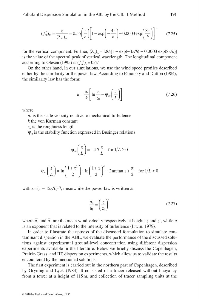
for the vertical component. Further, (λ m ) w = 1.8h[1 − exp(−4z/h) − 0.0003 exp(8z/h)]
is the value of the spectral peak of vertical wavelength. The longitudinal component
according to Olesen (1995) is (f m
* ) u = 0.67.
On the other hand, in our simulations, we use the wind speed profi les described
either by the similarity or the power law. According to Panofsky and Dutton (1984),
the similarity law has the form:
0
ln
m
u
z
z
u
k
z
L
∗ ⎡
⎤
⎛ ⎞
=
−ψ ⎜ ⎟
⎢
⎥
⎝ ⎠
⎣
⎦
(7.26)
where
u * is the scale velocity relative to mechanical turbulence
k the von Karman constant
z o is the roughness length
ψ m is the stability function expressed in Businger relations
4.7
for 1
0
m
z
z
L
L
L
⎛ ⎞
ψ
=−
≥
⎜ ⎟
⎝ ⎠
2
2
1
1
ln
ln
2 arctan
for 1
0
2
2
2
m
z
x
x
x
L
L
⎛
⎞
+
+
π
⎛ ⎞
⎛
⎞
ψ
=
+
−
+
<
⎜ ⎟
⎜
⎟
⎜
⎟
⎝ ⎠
⎝
⎠
⎝
⎠
with x = (1 − 15z/L) 1/4 , meanwhile the power law is written as
1
1
n
z
u
z
u
z
⎛ ⎞
= ⎜ ⎟
⎝ ⎠
(7.27)
where u
–
z and u
–
1 are the mean wind velocity respectively at heights z and z 1 , while n
is an exponent that is related to the intensity of turbulence (Irwin, 1979).
In order to illustrate the aptness of the discussed formulation to simulate contaminant dispersion in the ABL, we evaluate the performance of the discussed solutions against experimental ground-level concentration using different dispersion
experiments available in the literature. Below we briefl y discuss the Copenhagen,
Prairie-Grass, and IIT dispersion experiments, which allow us to validate the results
encountered by the mentioned solutions.
The fi rst experiment is carried out in the northern part of Copenhagen, described
by Gryning and Lyck (1984). It consisted of a tracer released without buoyancy
from a tower at a height of 115 m, and collection of tracer sampling units at the
© 2010 by Taylor and Francis Group, LLC
191
1
*
4
8
( )
0.55
1 exp
0.0003exp
( )
m w
m w
z
z
z
z
f
h
h
h
−
⎡
⎤
⎛ ⎞
⎛
⎞
⎛ ⎞
=
=
−
−
−
⎜ ⎟
⎜
⎟
⎜ ⎟
⎢
⎥
⎝ ⎠
⎝
⎠
⎝ ⎠
λ
⎣
⎦
(7.25)
for the vertical component. Further, (λ m ) w = 1.8h[1 − exp(−4z/h) − 0.0003 exp(8z/h)]
is the value of the spectral peak of vertical wavelength. The longitudinal component
according to Olesen (1995) is (f m
* ) u = 0.67.
On the other hand, in our simulations, we use the wind speed profi les described
either by the similarity or the power law. According to Panofsky and Dutton (1984),
the similarity law has the form:
0
ln
m
u
z
z
u
k
z
L
∗ ⎡
⎤
⎛ ⎞
=
−ψ ⎜ ⎟
⎢
⎥
⎝ ⎠
⎣
⎦
(7.26)
where
u * is the scale velocity relative to mechanical turbulence
k the von Karman constant
z o is the roughness length
ψ m is the stability function expressed in Businger relations
4.7
for 1
0
m
z
z
L
L
L
⎛ ⎞
ψ
=−
≥
⎜ ⎟
⎝ ⎠
2
2
1
1
ln
ln
2 arctan
for 1
0
2
2
2
m
z
x
x
x
L
L
⎛
⎞
+
+
π
⎛ ⎞
⎛
⎞
ψ
=
+
−
+
<
⎜ ⎟
⎜
⎟
⎜
⎟
⎝ ⎠
⎝
⎠
⎝
⎠
with x = (1 − 15z/L) 1/4 , meanwhile the power law is written as
1
1
n
z
u
z
u
z
⎛ ⎞
= ⎜ ⎟
⎝ ⎠
(7.27)
where u
–
z and u
–
1 are the mean wind velocity respectively at heights z and z 1 , while n
is an exponent that is related to the intensity of turbulence (Irwin, 1979).
In order to illustrate the aptness of the discussed formulation to simulate contaminant dispersion in the ABL, we evaluate the performance of the discussed solutions against experimental ground-level concentration using different dispersion
experiments available in the literature. Below we briefl y discuss the Copenhagen,
Prairie-Grass, and IIT dispersion experiments, which allow us to validate the results
encountered by the mentioned solutions.
The fi rst experiment is carried out in the northern part of Copenhagen, described
by Gryning and Lyck (1984). It consisted of a tracer released without buoyancy
from a tower at a height of 115 m, and collection of tracer sampling units at the
© 2010 by Taylor and Francis Group, LLC