

Mathematical Air Pollution Models: Eulerian Models
145
The Brookhaven sigmas (Smith, 1968), for which a power law is assumed (for
both σ y and σ z ), are written as
b
ax
σ =
(5.18)
where the coeffi cients a and b vary according to the stability classes.
Briggs’s sigmas (Briggs, 1973) distinguish between diffusion in the open country
and urban environment (Table 5.4).
More recently, the “sigmas” have been expressed as functions of continuous variables of atmospheric turbulence. Most of them are based on the approach proposed
by Pasquill (1971). He retained the essential features of Taylor’s statistical theory, but
evaluated the dispersion parameters in terms of the turbulence quantities and their
related timescale using the following expressions:
( )
σ = σ
L
/
y
v y
tS t T
(5.19a)
( )
σ = σ
L
/
z
w z
tS t T
(5.19b)
where
σ v and σ w are the standard deviations of the transversal and vertical components
of wind velocity
S y and S z are universal functions of the diffusion time t and Lagrangian timescale T L
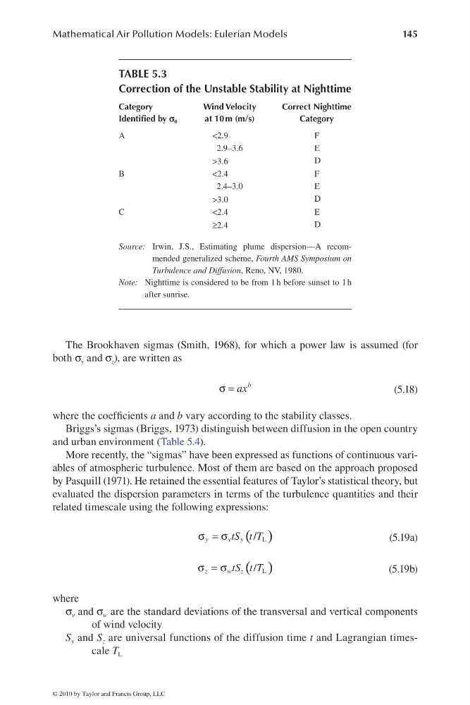
TABLE 5.3
Correction of the Unstable Stability at Nighttime
Category
Identifi ed by s q
Wind Velocity
at 10 m (m/s)
Correct Nighttime
Category
A
<2.9
F
2.9–3.6
E
>3.6
D
B
<2.4
F
2.4–3.0
E
>3.0
D
C
<2.4
E
≥2.4
D
Source: Irwin, J.S., Estimating plume dispersion—A recommended generalized scheme, Fourth AMS Symposium on
Turbulence and Diffusion, Reno, NV, 1980.
Note: Nighttime is considered to be from 1 h before sunset to 1 h
after sunrise.
© 2010 by Taylor and Francis Group, LLC
145
The Brookhaven sigmas (Smith, 1968), for which a power law is assumed (for
both σ y and σ z ), are written as
b
ax
σ =
(5.18)
where the coeffi cients a and b vary according to the stability classes.
Briggs’s sigmas (Briggs, 1973) distinguish between diffusion in the open country
and urban environment (Table 5.4).
More recently, the “sigmas” have been expressed as functions of continuous variables of atmospheric turbulence. Most of them are based on the approach proposed
by Pasquill (1971). He retained the essential features of Taylor’s statistical theory, but
evaluated the dispersion parameters in terms of the turbulence quantities and their
related timescale using the following expressions:
( )
σ = σ
L
/
y
v y
tS t T
(5.19a)
( )
σ = σ
L
/
z
w z
tS t T
(5.19b)
where
σ v and σ w are the standard deviations of the transversal and vertical components
of wind velocity
S y and S z are universal functions of the diffusion time t and Lagrangian timescale T L
TABLE 5.3
Correction of the Unstable Stability at Nighttime
Category
Identifi ed by s q
Wind Velocity
at 10 m (m/s)
Correct Nighttime
Category
A
<2.9
F
2.9–3.6
E
>3.6
D
B
<2.4
F
2.4–3.0
E
>3.0
D
C
<2.4
E
≥2.4
D
Source: Irwin, J.S., Estimating plume dispersion—A recommended generalized scheme, Fourth AMS Symposium on
Turbulence and Diffusion, Reno, NV, 1980.
Note: Nighttime is considered to be from 1 h before sunset to 1 h
after sunrise.
© 2010 by Taylor and Francis Group, LLC