

Parameterization of Convective Boundary Layer Turbulence and Clouds
97
of thermals, M = a u w u , with the vertical velocity standard deviation. Therefore, it
was assumed
,
w
M c σ
≈ σ
(4.58)
where c σ = 0.5, making the M formulation dependent on the standard deviation of the
vertical velocity σ w , like in the parcel initialization.
As previously mentioned, this scheme was developed to be applied in global models, namely, the ECMWF model, hence the use of empirical expressions is appealing
due to its computational economy. Accordingly, the standard deviation is computed
using the empirical expression, derived from observations, tank measurements, and
LES simulations (Holtslag and Moeng 1991):
1
1
3
3
2
1.26
0.6
1
,
w
i
i
u
z
z
w
w
z
z
∗
∗
∗
⎡
⎤
⎛
⎞
⎢
⎥
σ
⎛
⎞
⎛ ⎞
≅
+
−
⎜
⎟
⎢
⎥
⎜ ⎟
⎜
⎟
⎝ ⎠
⎝
⎠
⎝
⎠
⎢
⎥
⎣
⎦
(4.59)
where w * is the convective velocity scale, given by
1
3
( (
) ) .
v s i
w
g w
z
∗ = β θ
′ ′
(4.60)
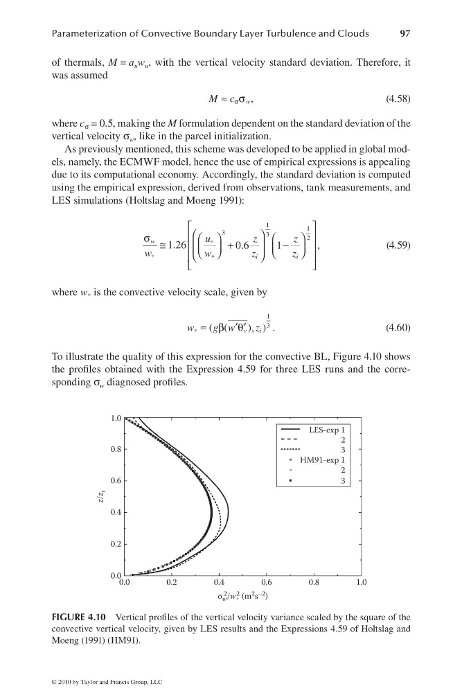
To illustrate the quality of this expression for the convective BL, Figure 4.10 shows
the profi les obtained with the Expression 4.59 for three LES runs and the corresponding σ w diagnosed profi les.
1.0
0.8
0.6
0.4
0.2
0.0
0.0
0.2
0.4
0.6
σ w
2 /w *
2 (m
2 s
–2 )
z/z
i
0.8
1.0
LES-exp 1
HM91-exp 1
2
3
2
3
FIGURE 4.10 Vertical profi les of the vertical velocity variance scaled by the square of the
convective vertical velocity, given by LES results and the Expressions 4.59 of Holtslag and
Moeng (1991) (HM91).
© 2010 by Taylor and Francis Group, LLC
97
of thermals, M = a u w u , with the vertical velocity standard deviation. Therefore, it
was assumed
,
w
M c σ
≈ σ
(4.58)
where c σ = 0.5, making the M formulation dependent on the standard deviation of the
vertical velocity σ w , like in the parcel initialization.
As previously mentioned, this scheme was developed to be applied in global models, namely, the ECMWF model, hence the use of empirical expressions is appealing
due to its computational economy. Accordingly, the standard deviation is computed
using the empirical expression, derived from observations, tank measurements, and
LES simulations (Holtslag and Moeng 1991):
1
1
3
3
2
1.26
0.6
1
,
w
i
i
u
z
z
w
w
z
z
∗
∗
∗
⎡
⎤
⎛
⎞
⎢
⎥
σ
⎛
⎞
⎛ ⎞
≅
+
−
⎜
⎟
⎢
⎥
⎜ ⎟
⎜
⎟
⎝ ⎠
⎝
⎠
⎝
⎠
⎢
⎥
⎣
⎦
(4.59)
where w * is the convective velocity scale, given by
1
3
( (
) ) .
v s i
w
g w
z
∗ = β θ
′ ′
(4.60)
To illustrate the quality of this expression for the convective BL, Figure 4.10 shows
the profi les obtained with the Expression 4.59 for three LES runs and the corresponding σ w diagnosed profi les.
1.0
0.8
0.6
0.4
0.2
0.0
0.0
0.2
0.4
0.6
σ w
2 /w *
2 (m
2 s
–2 )
z/z
i
0.8
1.0
LES-exp 1
HM91-exp 1
2
3
2
3
FIGURE 4.10 Vertical profi les of the vertical velocity variance scaled by the square of the
convective vertical velocity, given by LES results and the Expressions 4.59 of Holtslag and
Moeng (1991) (HM91).
© 2010 by Taylor and Francis Group, LLC