

96
Air Pollution and Turbulence: Modeling and Applications
4.4.2.2 The Mass-Flux Profi le
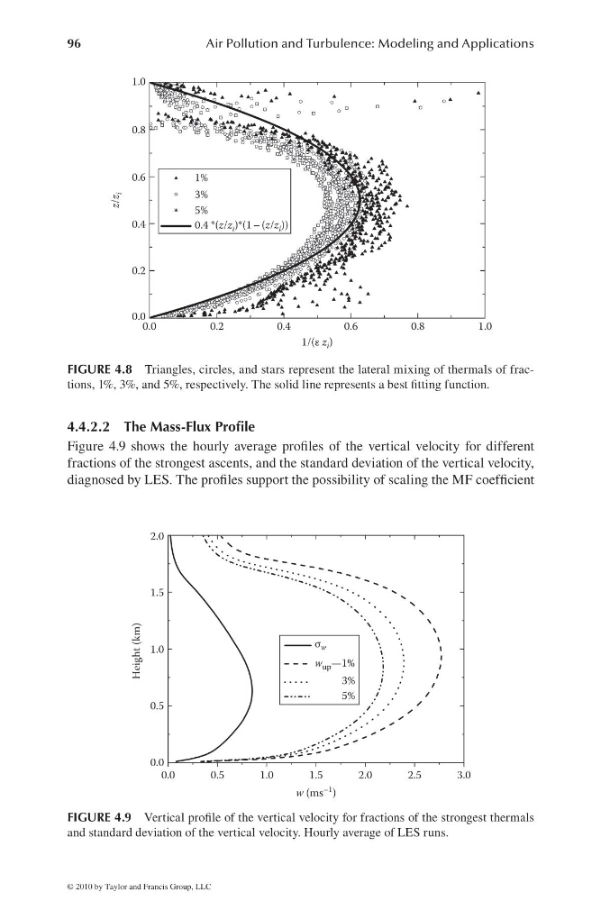
Figure 4.9 shows the hourly average profi les of the vertical velocity for different
fractions of the strongest ascents, and the standard deviation of the vertical velocity,
diagnosed by LES. The profi les support the possibility of scaling the MF coeffi cient
1.0
0.8
0.6
1%
3%
5%
0.4 *(z/z i )*(1 – (z/z i ))
0.4
0.2
0.0
0.0
0.2
0.4
1/(ε z i )
z/z
i
0.6
0.8
1.0
FIGURE 4.8 Triangles, circles, and stars represent the lateral mixing of thermals of fractions, 1%, 3%, and 5%, respectively. The solid line represents a best fi tting function.
2.0
1.5
1.0
Height (km)
w (ms
–1 )
0.5
0.0
0.0
0.5
1.0
1.5
2.0
2.5
3.0
σ w
w up —1%
3%
5%
FIGURE 4.9 Vertical profi le of the vertical velocity for fractions of the strongest thermals
and standard deviation of the vertical velocity. Hourly average of LES runs.
© 2010 by Taylor and Francis Group, LLC
Air Pollution and Turbulence: Modeling and Applications
4.4.2.2 The Mass-Flux Profi le
Figure 4.9 shows the hourly average profi les of the vertical velocity for different
fractions of the strongest ascents, and the standard deviation of the vertical velocity,
diagnosed by LES. The profi les support the possibility of scaling the MF coeffi cient
1.0
0.8
0.6
1%
3%
5%
0.4 *(z/z i )*(1 – (z/z i ))
0.4
0.2
0.0
0.0
0.2
0.4
1/(ε z i )
z/z
i
0.6
0.8
1.0
FIGURE 4.8 Triangles, circles, and stars represent the lateral mixing of thermals of fractions, 1%, 3%, and 5%, respectively. The solid line represents a best fi tting function.
2.0
1.5
1.0
Height (km)
w (ms
–1 )
0.5
0.0
0.0
0.5
1.0
1.5
2.0
2.5
3.0
σ w
w up —1%
3%
5%
FIGURE 4.9 Vertical profi le of the vertical velocity for fractions of the strongest thermals
and standard deviation of the vertical velocity. Hourly average of LES runs.
© 2010 by Taylor and Francis Group, LLC