

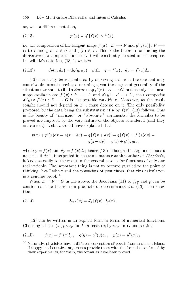
150
IX – Multivariate Differential and Integral Calculus
or, with a different notation,
p
(x) = g
[f (x)] ◦ f
(x) ,
(2.13)
i.e. the composition of the tangent maps f
(x) : E −→ F and g
[f (x)] : F −→
G to f and g at x ∈ U and f (x) ∈ V . This is the theorem for finding the
derivative of a composite function. It will constantly be used in this chapter.
In Leibniz’s notation, (13) is written
dp(x; dx) = dg(y; dy) with y = f (x) , dy = f
(x)dx .
(2.13’)
(13) can easily be remembered by observing that it is the one and only
conceivable formula having a meaning given the degree of generality of the
situation : we want to find a linear map p
(x) : E −→ G, and as only the linear
maps available are f
(x) : E −→ F and g
(y) : F −→ G, their composite
g
(y) ◦ f
(x) : E −→ G is the possible candidate . Moreover, as the result
sought should not depend on x, y must depend on it. The only possibility
proposed by the data being the substitution of y by f (x), (13) follows. This
is the beauty of “ intrinsic ” or “ absolute ” arguments : the formulas to be
proved are imposed by the very nature of the objects considered (and they
are correct). Leibniz would have explained that
p(x) + p
(x)dx = p(x + dx) = g [f (x + dx)] = g [f (x) + f
(x)dx] =
= g(y + dy) = g(y) + g
(y)dy ,
where y = f (x) and dy = f
(x)dx; hence (13’). Though this argument makes
no sense if dx is interpreted in the same manner as the author of Th´ eodic´ ee,
it leads as easily to the result in the general case as for functions of only one
real variable. The important thing is not to become puzzled to the point of
thinking, like Leibniz and the physicists of past times, that this calculation
is a genuine proof.
16
When E = F = G in the above, the Jacobians (11) of f, g and p can be
considered. The theorem on products of determinants and (13) then show
that
J g◦f (x) = J g [f (x)] J f (x) .
(2.14)
(12) can be written is an explicit form in terms of numerical functions.
Choosing a basis (b j ) 1≤j≤p for F , a basis (c k ) 1≤k≤q for G and setting
f (x) = f
j (x)b j , g(y) = g
k (y)c k , p(x) = p
k (x)c k
(2.15)
16 Naturally, physicists have a different conception of proofs from mathematicians:
if sloppy mathematical arguments provide them with the formulas confirmed by
their experiments, for them, the formulas have been proved.
IX – Multivariate Differential and Integral Calculus
or, with a different notation,
p
(x) = g
[f (x)] ◦ f
(x) ,
(2.13)
i.e. the composition of the tangent maps f
(x) : E −→ F and g
[f (x)] : F −→
G to f and g at x ∈ U and f (x) ∈ V . This is the theorem for finding the
derivative of a composite function. It will constantly be used in this chapter.
In Leibniz’s notation, (13) is written
dp(x; dx) = dg(y; dy) with y = f (x) , dy = f
(x)dx .
(2.13’)
(13) can easily be remembered by observing that it is the one and only
conceivable formula having a meaning given the degree of generality of the
situation : we want to find a linear map p
(x) : E −→ G, and as only the linear
maps available are f
(x) : E −→ F and g
(y) : F −→ G, their composite
g
(y) ◦ f
(x) : E −→ G is the possible candidate . Moreover, as the result
sought should not depend on x, y must depend on it. The only possibility
proposed by the data being the substitution of y by f (x), (13) follows. This
is the beauty of “ intrinsic ” or “ absolute ” arguments : the formulas to be
proved are imposed by the very nature of the objects considered (and they
are correct). Leibniz would have explained that
p(x) + p
(x)dx = p(x + dx) = g [f (x + dx)] = g [f (x) + f
(x)dx] =
= g(y + dy) = g(y) + g
(y)dy ,
where y = f (x) and dy = f
(x)dx; hence (13’). Though this argument makes
no sense if dx is interpreted in the same manner as the author of Th´ eodic´ ee,
it leads as easily to the result in the general case as for functions of only one
real variable. The important thing is not to become puzzled to the point of
thinking, like Leibniz and the physicists of past times, that this calculation
is a genuine proof.
16
When E = F = G in the above, the Jacobians (11) of f, g and p can be
considered. The theorem on products of determinants and (13) then show
that
J g◦f (x) = J g [f (x)] J f (x) .
(2.14)
(12) can be written is an explicit form in terms of numerical functions.
Choosing a basis (b j ) 1≤j≤p for F , a basis (c k ) 1≤k≤q for G and setting
f (x) = f
j (x)b j , g(y) = g
k (y)c k , p(x) = p
k (x)c k
(2.15)
16 Naturally, physicists have a different conception of proofs from mathematicians:
if sloppy mathematical arguments provide them with the formulas confirmed by
their experiments, for them, the formulas have been proved.