

300
III - Convergence: Continuous variables
y
o
g(y)
x
fig. 15.
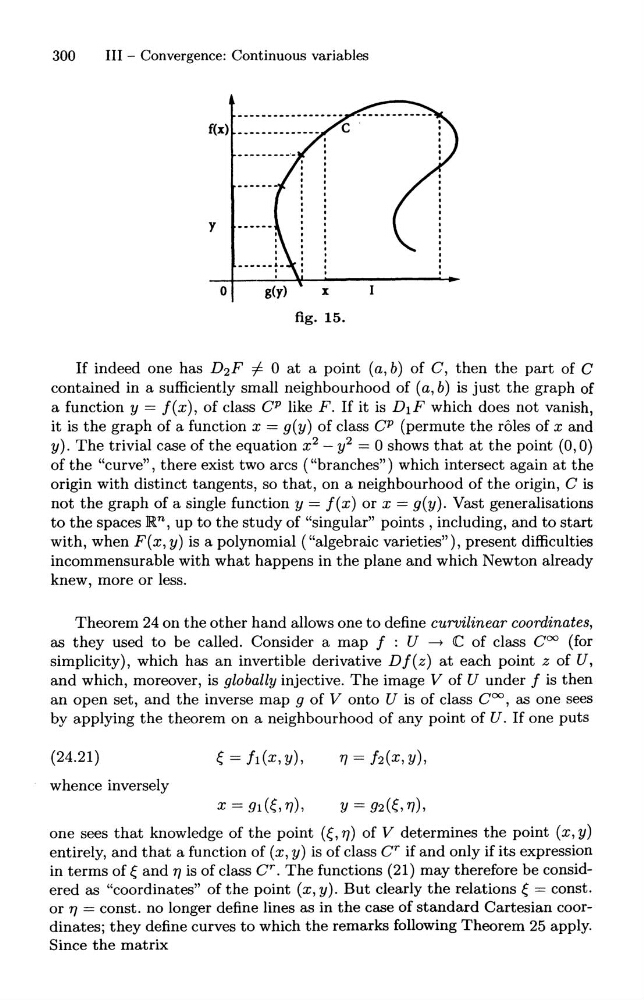
If indeed one has D2F =I- 0 at a point (a, b) of C, then the part of C
contained in a sufficiently small neighbourhood of (a, b) is just the graph of
a function y = J(x), of class CP like F. If it is D1F which does not vanish,
it is the graph of a function x = g(y) of class CP (permute the roles of x and
y). The trivial case of the equation x 2 - y2 = 0 shows that at the point (0,0)
of the "curve", there exist two arcs ("branches") which intersect again at the
origin with distinct tangents, so that, on a neighbourhood of the origin, C is
not the graph of a single function y = J(x) or x = g(y). Vast generalisations
to the spaces lR,n, up to the study of "singular" points, including, and to start
with, when F(x, y) is a polynomial ("algebraic varieties"), present difficulties
incommensurable with what happens in the plane and which Newton already
knew, more or less.
Theorem 24 on the other hand allows one to define curvilinear coordinates,
as they used to be called. Consider a map J : U ----+ C of class Coo (for
simplicity), which has an invertible derivative DJ(z) at each point z of U,
and which, moreover, is globally injective. The image V of U under J is then
an open set, and the inverse map 9 of V onto U is of class Coo, as one sees
by applying the theorem on a neighbourhood of any point of U. If one puts
(24.21 )
~ = hex, y),
TJ = hex, y),
whence inversely
x = g1 (~, TJ),
one sees that knowledge of the point (~, TJ) of V determines the point (x, y)
entirely, and that a function of (x, y) is of class C r if and only if its expression
in terms of ~ and TJ is of class cr. The functions (21) may therefore be considered as "coordinates" of the point (x, y). But clearly the relations ~ = const.
or TJ = const. no longer define lines as in the case of standard Cartesian coordinates; they define curves to which the remarks following Theorem 25 apply.
Since the matrix
III - Convergence: Continuous variables
y
o
g(y)
x
fig. 15.
If indeed one has D2F =I- 0 at a point (a, b) of C, then the part of C
contained in a sufficiently small neighbourhood of (a, b) is just the graph of
a function y = J(x), of class CP like F. If it is D1F which does not vanish,
it is the graph of a function x = g(y) of class CP (permute the roles of x and
y). The trivial case of the equation x 2 - y2 = 0 shows that at the point (0,0)
of the "curve", there exist two arcs ("branches") which intersect again at the
origin with distinct tangents, so that, on a neighbourhood of the origin, C is
not the graph of a single function y = J(x) or x = g(y). Vast generalisations
to the spaces lR,n, up to the study of "singular" points, including, and to start
with, when F(x, y) is a polynomial ("algebraic varieties"), present difficulties
incommensurable with what happens in the plane and which Newton already
knew, more or less.
Theorem 24 on the other hand allows one to define curvilinear coordinates,
as they used to be called. Consider a map J : U ----+ C of class Coo (for
simplicity), which has an invertible derivative DJ(z) at each point z of U,
and which, moreover, is globally injective. The image V of U under J is then
an open set, and the inverse map 9 of V onto U is of class Coo, as one sees
by applying the theorem on a neighbourhood of any point of U. If one puts
(24.21 )
~ = hex, y),
TJ = hex, y),
whence inversely
x = g1 (~, TJ),
one sees that knowledge of the point (~, TJ) of V determines the point (x, y)
entirely, and that a function of (x, y) is of class C r if and only if its expression
in terms of ~ and TJ is of class cr. The functions (21) may therefore be considered as "coordinates" of the point (x, y). But clearly the relations ~ = const.
or TJ = const. no longer define lines as in the case of standard Cartesian coordinates; they define curves to which the remarks following Theorem 25 apply.
Since the matrix