

Natural and Anthropogenic Mercury Sources
23
Hg, while soils above that concentration emit mercury depending on the Hg(o)
concentration in the overlying air (Kim et al. 1995); even if the mechanisms of
emission and absorption may not be the same). A similar compensation point
concept has also been reported for vegetation (Hanson et al. 1995).
Other properties whose gradients influence mercury transfer across the airsurface boundary include temperature, pressure and moisture. Therefore, soil
temperature correlates well with mercury emission (Kim et al. 1995), higher
fluxes are observed at low barometric pressure (McNerney and Buseck 1973) (the
soil air is "sucked out" of the soil), and soils emit more mercury in the moist (not
flooded) state compared to the dry state (WallschHiger et al. 1997b). In fact, one
study of forest soils demonstrated that fluxes could change from net emission to
net deposition depending on the soils moisture status (Advokaat and Lindberg
1996). In addition, any condition that favors conversion of oxidized Hg(II) to
volatile mercury species in the investigated compartment, e.g., sunlight (Amyot
et al. 1994; Carpi and Lindberg 1997) or bacterial activity, increases Hg fluxes to
the atmosphere. Also, processes that accelerate the transport across the boundary
layer increase the Hg flux. For example, high turbulence or winds peed conditions
(Kim et al. 1995) that transport the liberated Hg away from the surface produce
an elevated volatilization rate. Similarly, wave breaking increases the surface area
and thereby the overall Hg flux from oceans to the atmosphere (Baeyens et al.
1991).
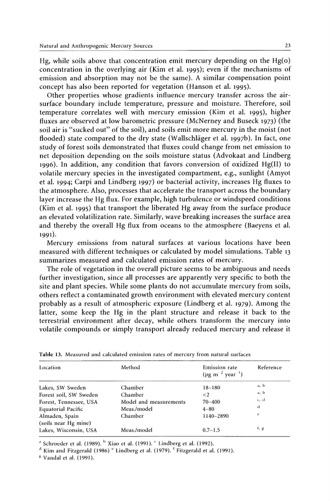
Mercury emissions from natural surfaces at various locations have been
measured with different techniques or calculated by model simulations. Table 13
summarizes measured and calculated emission rates of mercury.
The role of vegetation in the overall picture seems to be ambiguous and needs
further investigation, since all processes are apparently very specific to both the
site and plant species. While some plants do not accumulate mercury from soils,
others reflect a contaminated growth environment with elevated mercury content
probably as a result of atmospheric exposure (Lindberg et al. 1979). Among the
latter, some keep the Hg in the plant structure and release it back to the
terrestrial environment after decay, while others transform the mercury into
volatile compounds or simply transport already reduced mercury and release it
Table 13. Measured and calculated emission rates of mercury from natural surfaces
Location
Method
Emission rate
(fig m 2 year ')
Lakes, SW Sweden
Chamber
18-180
Forest soil, SW Sweden
Chamber
<2
Forest, Tennessee, USA
Model and measurements
70-400
Equatorial Pacific
Meas.lmodel
4-80
Almaden, Spain
Chamber
1140-2890
(soils near Hg mine)
Lakes, Wisconsin, USA
Meas.lmodel
0.7-\.5
a Schroeder et al. (1989). h Xiao et al. (1991). < Lindberg et al. (1992).
" Kim and Fitzgerald (1986) e Lindberg et al. (1979). f Fitzgerald et al. (1991).
g Vandal et al. (1991).
Reference
r. g
23
Hg, while soils above that concentration emit mercury depending on the Hg(o)
concentration in the overlying air (Kim et al. 1995); even if the mechanisms of
emission and absorption may not be the same). A similar compensation point
concept has also been reported for vegetation (Hanson et al. 1995).
Other properties whose gradients influence mercury transfer across the airsurface boundary include temperature, pressure and moisture. Therefore, soil
temperature correlates well with mercury emission (Kim et al. 1995), higher
fluxes are observed at low barometric pressure (McNerney and Buseck 1973) (the
soil air is "sucked out" of the soil), and soils emit more mercury in the moist (not
flooded) state compared to the dry state (WallschHiger et al. 1997b). In fact, one
study of forest soils demonstrated that fluxes could change from net emission to
net deposition depending on the soils moisture status (Advokaat and Lindberg
1996). In addition, any condition that favors conversion of oxidized Hg(II) to
volatile mercury species in the investigated compartment, e.g., sunlight (Amyot
et al. 1994; Carpi and Lindberg 1997) or bacterial activity, increases Hg fluxes to
the atmosphere. Also, processes that accelerate the transport across the boundary
layer increase the Hg flux. For example, high turbulence or winds peed conditions
(Kim et al. 1995) that transport the liberated Hg away from the surface produce
an elevated volatilization rate. Similarly, wave breaking increases the surface area
and thereby the overall Hg flux from oceans to the atmosphere (Baeyens et al.
1991).
Mercury emissions from natural surfaces at various locations have been
measured with different techniques or calculated by model simulations. Table 13
summarizes measured and calculated emission rates of mercury.
The role of vegetation in the overall picture seems to be ambiguous and needs
further investigation, since all processes are apparently very specific to both the
site and plant species. While some plants do not accumulate mercury from soils,
others reflect a contaminated growth environment with elevated mercury content
probably as a result of atmospheric exposure (Lindberg et al. 1979). Among the
latter, some keep the Hg in the plant structure and release it back to the
terrestrial environment after decay, while others transform the mercury into
volatile compounds or simply transport already reduced mercury and release it
Table 13. Measured and calculated emission rates of mercury from natural surfaces
Location
Method
Emission rate
(fig m 2 year ')
Lakes, SW Sweden
Chamber
18-180
Forest soil, SW Sweden
Chamber
<2
Forest, Tennessee, USA
Model and measurements
70-400
Equatorial Pacific
Meas.lmodel
4-80
Almaden, Spain
Chamber
1140-2890
(soils near Hg mine)
Lakes, Wisconsin, USA
Meas.lmodel
0.7-\.5
a Schroeder et al. (1989). h Xiao et al. (1991). < Lindberg et al. (1992).
" Kim and Fitzgerald (1986) e Lindberg et al. (1979). f Fitzgerald et al. (1991).
g Vandal et al. (1991).
Reference
r. g