

Estimation of Gaseous Mercury Emissions in Germany
387
location of the theoretical measurements inside the plume was chosen in a crosswind direction for different distances from the sources in a downwind direction.
For each cross-section three or four data points were selected. The next step of
the performance test was running the inverse modelling procedure for a different
number of theoretical measurements. For the minimizing procedure maximum
values of the source strengths were defined to be a factor of 3 of the theoretical
source strengths. These maximum emissions were chosen as starting values. The
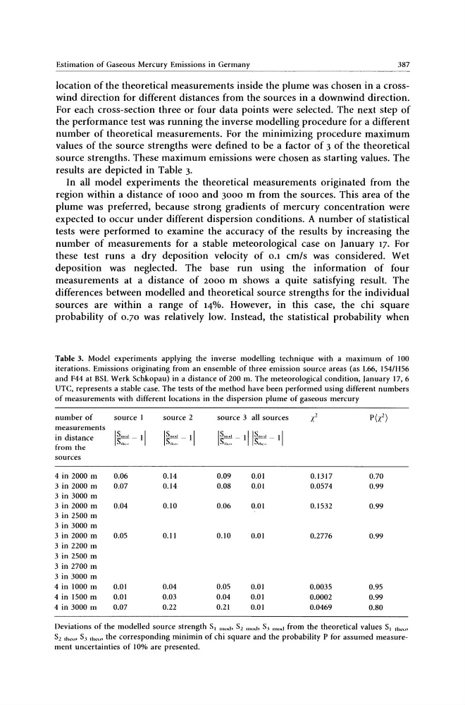
results are depicted in Table 3.
In all model experiments the theoretical measurements originated from the
region within a distance of 1000 and 3000 m from the sources. This area of the
plume was preferred, because strong gradients of mercury concentration were
expected to occur under different dispersion conditions. A number of statistical
tests were performed to examine the accuracy of the results by increasing the
number of measurements for a stable meteorological case on January 17. For
these test runs a dry deposition velocity of 0.1 cm/s was considered. Wet
deposition was neglected. The base run using the information of four
measurements at a distance of 2000 m shows a quite satisfying result. The
differences between modelled and theoretical source strengths for the individual
sources are within a range of 14%. However, in this case, the chi square
probability of 0.70 was relatively low. Instead, the statistical probability when
Table 3. Model experiments applying the inverse modelling technique with a maximum of 100
iterations. Emissions originating from an ensemble of three emission source areas (as L66, 154/H56
and F44 at BSL Werk Schkopau) in a distance of 200 m. The meteorological condition, January 17,6
UTe, represents a stable case. The tests of the method have been performed using different numbers
of measurements with different locations in the dispersion plume of gaseous mercury
number of
source I
source 2
source 3 all sources
X 2
P(X 2 )
measurements
in distance
I~-II I~-II
I~ IllS""'" II
from the
~sources
4 in 2000 m
0.06
0.14
0.09
0.01
0.1317
0.70
3 in 2000 m
0.07
0.14
0.08
0.01
0.0574
0.99
3 in 3000 m
3 in 2000 m
0.04
0.10
0.06
0.01
0.1532
0.99
3 in 2500 m
3 in 3000 m
3 in 2000 m
0.05
0.11
0.10
0.01
0.2776
0.99
3 in 2200 m
3 in 2500 m
3 in 2700 m
3 in 3000 m
4 in 1000 m
0.01
0.04
0.05
0.01
0.0035
0.95
4 in 1500 m
0.01
0.03
0.04
0.01
0.0002
0.99
4 in 3000 m
0.07
0.22
0.21
0.01
0.0469
0.80
Deviations of the modelled source strength S, ",od, S2 "'mb Sj "",,' from the theoretical values S, ,hen'
S2 ,he'" Sj ,heo' the corresponding minimin of chi square and the probability P for assumed measurement uncertainties of 10% are presented.
387
location of the theoretical measurements inside the plume was chosen in a crosswind direction for different distances from the sources in a downwind direction.
For each cross-section three or four data points were selected. The next step of
the performance test was running the inverse modelling procedure for a different
number of theoretical measurements. For the minimizing procedure maximum
values of the source strengths were defined to be a factor of 3 of the theoretical
source strengths. These maximum emissions were chosen as starting values. The
results are depicted in Table 3.
In all model experiments the theoretical measurements originated from the
region within a distance of 1000 and 3000 m from the sources. This area of the
plume was preferred, because strong gradients of mercury concentration were
expected to occur under different dispersion conditions. A number of statistical
tests were performed to examine the accuracy of the results by increasing the
number of measurements for a stable meteorological case on January 17. For
these test runs a dry deposition velocity of 0.1 cm/s was considered. Wet
deposition was neglected. The base run using the information of four
measurements at a distance of 2000 m shows a quite satisfying result. The
differences between modelled and theoretical source strengths for the individual
sources are within a range of 14%. However, in this case, the chi square
probability of 0.70 was relatively low. Instead, the statistical probability when
Table 3. Model experiments applying the inverse modelling technique with a maximum of 100
iterations. Emissions originating from an ensemble of three emission source areas (as L66, 154/H56
and F44 at BSL Werk Schkopau) in a distance of 200 m. The meteorological condition, January 17,6
UTe, represents a stable case. The tests of the method have been performed using different numbers
of measurements with different locations in the dispersion plume of gaseous mercury
number of
source I
source 2
source 3 all sources
X 2
P(X 2 )
measurements
in distance
I~-II I~-II
I~ IllS""'" II
from the
~sources
4 in 2000 m
0.06
0.14
0.09
0.01
0.1317
0.70
3 in 2000 m
0.07
0.14
0.08
0.01
0.0574
0.99
3 in 3000 m
3 in 2000 m
0.04
0.10
0.06
0.01
0.1532
0.99
3 in 2500 m
3 in 3000 m
3 in 2000 m
0.05
0.11
0.10
0.01
0.2776
0.99
3 in 2200 m
3 in 2500 m
3 in 2700 m
3 in 3000 m
4 in 1000 m
0.01
0.04
0.05
0.01
0.0035
0.95
4 in 1500 m
0.01
0.03
0.04
0.01
0.0002
0.99
4 in 3000 m
0.07
0.22
0.21
0.01
0.0469
0.80
Deviations of the modelled source strength S, ",od, S2 "'mb Sj "",,' from the theoretical values S, ,hen'
S2 ,he'" Sj ,heo' the corresponding minimin of chi square and the probability P for assumed measurement uncertainties of 10% are presented.