

Estimation of Gaseous Mercury Emissions in Germany
383
The model, which is an extension of the elementary Gaussian model,
essentially is an Eulerian model, whose parametrizations are more closely
related to the transport properties of the atmosphere. It has been shown (Eppel
et a1. 1991) that the model also performs a quite realistic dispersion for episodes
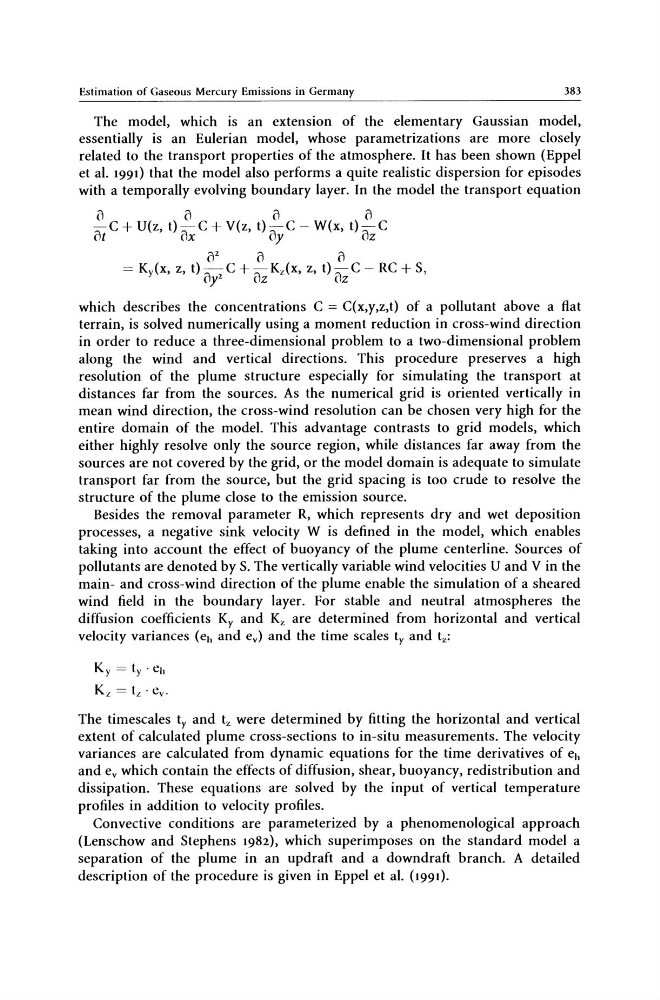
with a temporally evolving boundary layer. In the model the transport equation
o
0
0
0
ot C + U(z, t) ox C + V(z, t) oy C - W(x, t) OZ C
0 2
0
0
= Ky(x, z, t);-C + ;-KAx, z, t);-C - RC + S,
\ly2
\IZ
uZ
which describes the concentrations C = C(x,y,z,t) of a pollutant above a flat
terrain, is solved numerically using a moment reduction in cross-wind direction
in order to reduce a three-dimensional problem to a two-dimensional problem
along the wind and vertical directions. This procedure preserves a high
resolution of the plume structure especially for simulating the transport at
distances far from the sources. As the numerical grid is oriented vertically in
mean wind direction, the cross-wind resolution can be chosen very high for the
entire domain of the modeL This advantage contrasts to grid models, which
either highly resolve only the source region, while distances far away from the
sources are not covered by the grid, or the model domain is adequate to simulate
transport far from the source, but the grid spacing is too crude to resolve the
structure of the plume close to the emission source.
Besides the removal parameter R, which represents dry and wet deposition
processes, a negative sink velocity W is defined in the model, which enables
taking into account the effect of buoyancy of the plume centerline. Sources of
pollutants are denoted by S. The vertically variable wind velocities U and V in the
main- and cross-wind direction of the plume enable the simulation of a sheared
wind field in the boundary layer. For stable and neutral atmospheres the
diffusion coefficients Ky and Kz are determined from horizontal and vertical
velocity variances (eh and ey} and the time scales ty and tz :
Ky = ty . eh
KL = tL . ev·
The timescales ty and tz were determined by fitting the horizontal and vertical
extent of calculated plume cross-sections to in-situ measurements. The velocity
variances are calculated from dynamic equations for the time derivatives of eh
and ev which contain the effects of diffusion, shear, buoyancy, redistribution and
dissipation. These equations are solved by the input of vertical temperature
profiles in addition to velocity profiles.
Convective conditions are parameterized by a phenomenological approach
(Lenschow and Stephens 1982), which superimposes on the standard model a
separation of the plume in an updraft and a downdraft branch. A detailed
description of the procedure is given in Eppel et aL (1991).
383
The model, which is an extension of the elementary Gaussian model,
essentially is an Eulerian model, whose parametrizations are more closely
related to the transport properties of the atmosphere. It has been shown (Eppel
et a1. 1991) that the model also performs a quite realistic dispersion for episodes
with a temporally evolving boundary layer. In the model the transport equation
o
0
0
0
ot C + U(z, t) ox C + V(z, t) oy C - W(x, t) OZ C
0 2
0
0
= Ky(x, z, t);-C + ;-KAx, z, t);-C - RC + S,
\ly2
\IZ
uZ
which describes the concentrations C = C(x,y,z,t) of a pollutant above a flat
terrain, is solved numerically using a moment reduction in cross-wind direction
in order to reduce a three-dimensional problem to a two-dimensional problem
along the wind and vertical directions. This procedure preserves a high
resolution of the plume structure especially for simulating the transport at
distances far from the sources. As the numerical grid is oriented vertically in
mean wind direction, the cross-wind resolution can be chosen very high for the
entire domain of the modeL This advantage contrasts to grid models, which
either highly resolve only the source region, while distances far away from the
sources are not covered by the grid, or the model domain is adequate to simulate
transport far from the source, but the grid spacing is too crude to resolve the
structure of the plume close to the emission source.
Besides the removal parameter R, which represents dry and wet deposition
processes, a negative sink velocity W is defined in the model, which enables
taking into account the effect of buoyancy of the plume centerline. Sources of
pollutants are denoted by S. The vertically variable wind velocities U and V in the
main- and cross-wind direction of the plume enable the simulation of a sheared
wind field in the boundary layer. For stable and neutral atmospheres the
diffusion coefficients Ky and Kz are determined from horizontal and vertical
velocity variances (eh and ey} and the time scales ty and tz :
Ky = ty . eh
KL = tL . ev·
The timescales ty and tz were determined by fitting the horizontal and vertical
extent of calculated plume cross-sections to in-situ measurements. The velocity
variances are calculated from dynamic equations for the time derivatives of eh
and ev which contain the effects of diffusion, shear, buoyancy, redistribution and
dissipation. These equations are solved by the input of vertical temperature
profiles in addition to velocity profiles.
Convective conditions are parameterized by a phenomenological approach
(Lenschow and Stephens 1982), which superimposes on the standard model a
separation of the plume in an updraft and a downdraft branch. A detailed
description of the procedure is given in Eppel et aL (1991).