

Wind Within Crop Canopies
73
top of the canopy u(h) is equal to u(h) computed from Eq. (5.1), thus
matching the two profiles at the top of the canopy. The value for a in Fig.
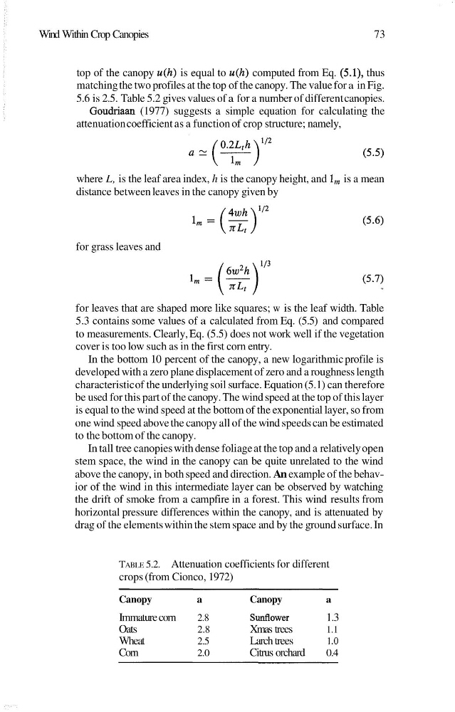
5.6 is 2.5. Table 5.2 gives values of a for a number of different canopies.
Goudriaan (1977) suggests a simple equation for calculating the
attenuation coefficient as a function of crop structure; namely,
where L, is the leaf area index, h is the canopy height, and 1, is a mean
distance between leaves in the canopy given by
for grass leaves and
for leaves that are shaped more like squares; w is the leaf width. Table
5.3 contains some values of a calculated from Eq. (5.5) and compared
to measurements. Clearly, Eq. (5.5) does not work well if the vegetation
cover is too low such as in the first corn entry.
In the bottom 10 percent of the canopy, a new logarithmic profile is
developed with a zero plane displacement of zero and a roughness length
characteristic of the underlying soil surface. Equation (5.1) can therefore
be used for this part of the canopy. The wind speed at the top of this layer
is equal to the wind speed at the bottom of the exponential layer, so from
one wind speed above the canopy all of the wind speeds can be estimated
to the bottom of the canopy.
In tall tree canopies with dense foliage at the top and a relatively open
stem space, the wind in the canopy can be quite unrelated to the wind
above the canopy, in both speed and direction. An example of the behavior of the wind in this intermediate layer can be observed by watching
the drift of smoke from a campfire in a forest. This wind results from
horizontal pressure differences within the canopy, and is attenuated by
drag of the elements within the stem space and by the ground surface. In
TABLE 5.2. Attenuation coefficients for different
crops (from Cionco, 1972)
Canopy
a
Canopy
a
Immature corn
2.8
Sunflower
1.3
Oats
2.8
Xmas trees
1.1
Wheat
2.5
Larch trees
1 .O
Corn
2.0
Citrus orchard
0.4
73
top of the canopy u(h) is equal to u(h) computed from Eq. (5.1), thus
matching the two profiles at the top of the canopy. The value for a in Fig.
5.6 is 2.5. Table 5.2 gives values of a for a number of different canopies.
Goudriaan (1977) suggests a simple equation for calculating the
attenuation coefficient as a function of crop structure; namely,
where L, is the leaf area index, h is the canopy height, and 1, is a mean
distance between leaves in the canopy given by
for grass leaves and
for leaves that are shaped more like squares; w is the leaf width. Table
5.3 contains some values of a calculated from Eq. (5.5) and compared
to measurements. Clearly, Eq. (5.5) does not work well if the vegetation
cover is too low such as in the first corn entry.
In the bottom 10 percent of the canopy, a new logarithmic profile is
developed with a zero plane displacement of zero and a roughness length
characteristic of the underlying soil surface. Equation (5.1) can therefore
be used for this part of the canopy. The wind speed at the top of this layer
is equal to the wind speed at the bottom of the exponential layer, so from
one wind speed above the canopy all of the wind speeds can be estimated
to the bottom of the canopy.
In tall tree canopies with dense foliage at the top and a relatively open
stem space, the wind in the canopy can be quite unrelated to the wind
above the canopy, in both speed and direction. An example of the behavior of the wind in this intermediate layer can be observed by watching
the drift of smoke from a campfire in a forest. This wind results from
horizontal pressure differences within the canopy, and is attenuated by
drag of the elements within the stem space and by the ground surface. In
TABLE 5.2. Attenuation coefficients for different
crops (from Cionco, 1972)
Canopy
a
Canopy
a
Immature corn
2.8
Sunflower
1.3
Oats
2.8
Xmas trees
1.1
Wheat
2.5
Larch trees
1 .O
Corn
2.0
Citrus orchard
0.4