

Conductances for Heat and Mass Transfer
z ~ .
However, the process of momentum exchange within the canopy differs from the scalar exchange processes (Garratt and Hicks, 1973), and
these differences can be modeled by adjusting the scalar roughness parameters. For our computations of aerodynamic conductance we assume
that:
ZH = Zv = 0 . 2 ~ ~ .
(7.19)
7.5 Fetch and Buoyancy
Now that we have equations describing turbulent transport, we need to
look briefly at their limitations. We started by assuming that the wind was
at a steady state with the surface (that there were no horizontal gradients).
When wind passes from one type of surface to another it must travel some
distance before a layer of air, solely influenced by the new surface, is built
up. The height of influence increases with downwind distance. The length
of uniform surface over which the wind has blown is termed fetch, and
the wind can usually be assumed to be 90 percent or more equilibrated
with the new surface to heights of 0.01 x fetch. Thus, at a distance 1000
m downwind from the edge of a uniform field of grain, expect the wind
profile equations to be valid to heights of around 10 m.
The effect of thermally produced turbulence on transport was alluded
to earlier, but its quantitative description was not given. The equations
derived to this point apply only for mechanically produced turbulence, so
they are appropriate only for adiabatic conditions. Strong heating of the
air near the surface of the earth causes overturning of the air layers, with
resultant increases in turbulence and mixing. Conversely, strong cooling
of these air layers suppresses mixing and turbulence. Thus convective
production or suppression of turbulence is directly related to sensible
heat flux (H) at the surface. When H is positive (surface warmer than
the air) the atmosphere is said to be unstable, and mixing is enhanced.
When H is negative, the atmosphere is said to be stable, and mixing
is suppressed by thermal stratification. When surface heating or cooling
occurs, corrections to Eqs. (7.16) through (7.18) are made and referred
to as "diabatic corrections."
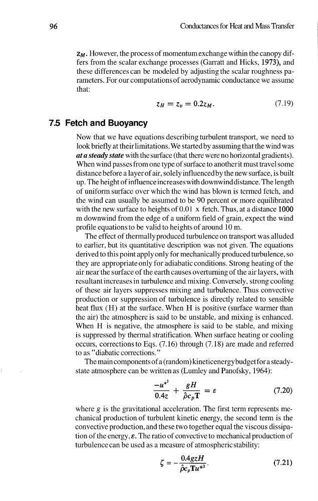
The main components of a (random) kinetic energy budget for a steadystate atmosphere can be written as (Lumley and Panofsky, 1964):
where g is the gravitational acceleration. The first term represents mechanical production of turbulent kinetic energy, the second term is the
convective production, and these two together equal the viscous dissipation of the energy, 8. The ratio of convective to mechanical production of
turbulence can be used as a measure of atmospheric stability:
z ~ .
However, the process of momentum exchange within the canopy differs from the scalar exchange processes (Garratt and Hicks, 1973), and
these differences can be modeled by adjusting the scalar roughness parameters. For our computations of aerodynamic conductance we assume
that:
ZH = Zv = 0 . 2 ~ ~ .
(7.19)
7.5 Fetch and Buoyancy
Now that we have equations describing turbulent transport, we need to
look briefly at their limitations. We started by assuming that the wind was
at a steady state with the surface (that there were no horizontal gradients).
When wind passes from one type of surface to another it must travel some
distance before a layer of air, solely influenced by the new surface, is built
up. The height of influence increases with downwind distance. The length
of uniform surface over which the wind has blown is termed fetch, and
the wind can usually be assumed to be 90 percent or more equilibrated
with the new surface to heights of 0.01 x fetch. Thus, at a distance 1000
m downwind from the edge of a uniform field of grain, expect the wind
profile equations to be valid to heights of around 10 m.
The effect of thermally produced turbulence on transport was alluded
to earlier, but its quantitative description was not given. The equations
derived to this point apply only for mechanically produced turbulence, so
they are appropriate only for adiabatic conditions. Strong heating of the
air near the surface of the earth causes overturning of the air layers, with
resultant increases in turbulence and mixing. Conversely, strong cooling
of these air layers suppresses mixing and turbulence. Thus convective
production or suppression of turbulence is directly related to sensible
heat flux (H) at the surface. When H is positive (surface warmer than
the air) the atmosphere is said to be unstable, and mixing is enhanced.
When H is negative, the atmosphere is said to be stable, and mixing
is suppressed by thermal stratification. When surface heating or cooling
occurs, corrections to Eqs. (7.16) through (7.18) are made and referred
to as "diabatic corrections."
The main components of a (random) kinetic energy budget for a steadystate atmosphere can be written as (Lumley and Panofsky, 1964):
where g is the gravitational acceleration. The first term represents mechanical production of turbulent kinetic energy, the second term is the
convective production, and these two together equal the viscous dissipation of the energy, 8. The ratio of convective to mechanical production of
turbulence can be used as a measure of atmospheric stability: