

J-2 Gauss surface normal coordinates: case study ellipsoid-of-revolution 645
ν(x 5 )
ν(x 3 )
ν(x 4 )
ν(x 2 )
ν(x 1 )
e1
e3
ν(x 5 )
ν(x 3 )
ν(x 4 )
ν(x 2 )
ν(x 1 )
Gauss map
↓
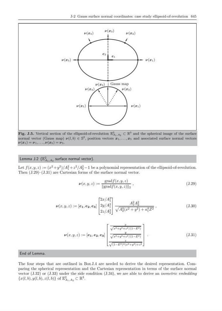
Fig. J.5. Vertical section of the ellipsoid-of-revolution E
2
A 1 ,A 2 ⊂ R
3 and the spherical image of the surface
normal vector (Gauss map) ν(l, b) ∈ S
2 , position vectors x 1 , . . . , x 5 and associated surface normal vectors
ν(x 1 ) = ν 1 , . . . , ν(x 5 ) = ν 5 .
Lemma J.2 (E
2
A 1 ,A 2
surface normal vector).
Let f (x, y, z) := (x
2 + y
2 )/A
2
1 + z
2 /A
2
2 − 1 be a polynomial representation of the ellipsoid-of-revolution.
Then (J.29)–(J.31) are Cartesian forms of the surface normal vector.
ν(x, y, z) :=
gradf (x, y, z)
gradf (x, y, z) 2
,
(J.29)
ν(x, y, z) := [e 1 , e 2 , e 3 ]
⎡
⎢
⎣
2x/A
2
1
2y/A
2
1
2z/A
2
2
⎤
⎥
⎦
A
2
1 A
2
2
A 4
2 (x 2 + y 2 ) + a 4
1 Z 2
,
(J.30)
ν(x, y, z) := [e 1 , e 2 , e 3 ]
⎡
⎢
⎢
⎢
⎣
x
√
x 2 +y 2 +z 2 /(1−E 2 )
y
√
x 2 +y 2 +z 2 /(1−E 2 )
z
√
(1−E 2 ) 2 (x 2 +y 2 )+z 2
⎤
⎥
⎥
⎥
⎦
.
(J.31)
End of Lemma.
The four steps that are outlined in Box J.4 are needed to derive the desired representation. Comparing the spherical representation and the Cartesian representation in terms of the surface normal
vector (J.32) or (J.33) under the side condition (J.34), we are able to derive an isometric embedding
{x(l, b), y(l, b), z(l, b)} of E
2
A 1 ,A 2
⊂ R
3 .
ν(x 5 )
ν(x 3 )
ν(x 4 )
ν(x 2 )
ν(x 1 )
e1
e3
ν(x 5 )
ν(x 3 )
ν(x 4 )
ν(x 2 )
ν(x 1 )
Gauss map
↓
Fig. J.5. Vertical section of the ellipsoid-of-revolution E
2
A 1 ,A 2 ⊂ R
3 and the spherical image of the surface
normal vector (Gauss map) ν(l, b) ∈ S
2 , position vectors x 1 , . . . , x 5 and associated surface normal vectors
ν(x 1 ) = ν 1 , . . . , ν(x 5 ) = ν 5 .
Lemma J.2 (E
2
A 1 ,A 2
surface normal vector).
Let f (x, y, z) := (x
2 + y
2 )/A
2
1 + z
2 /A
2
2 − 1 be a polynomial representation of the ellipsoid-of-revolution.
Then (J.29)–(J.31) are Cartesian forms of the surface normal vector.
ν(x, y, z) :=
gradf (x, y, z)
gradf (x, y, z) 2
,
(J.29)
ν(x, y, z) := [e 1 , e 2 , e 3 ]
⎡
⎢
⎣
2x/A
2
1
2y/A
2
1
2z/A
2
2
⎤
⎥
⎦
A
2
1 A
2
2
A 4
2 (x 2 + y 2 ) + a 4
1 Z 2
,
(J.30)
ν(x, y, z) := [e 1 , e 2 , e 3 ]
⎡
⎢
⎢
⎢
⎣
x
√
x 2 +y 2 +z 2 /(1−E 2 )
y
√
x 2 +y 2 +z 2 /(1−E 2 )
z
√
(1−E 2 ) 2 (x 2 +y 2 )+z 2
⎤
⎥
⎥
⎥
⎦
.
(J.31)
End of Lemma.
The four steps that are outlined in Box J.4 are needed to derive the desired representation. Comparing the spherical representation and the Cartesian representation in terms of the surface normal
vector (J.32) or (J.33) under the side condition (J.34), we are able to derive an isometric embedding
{x(l, b), y(l, b), z(l, b)} of E
2
A 1 ,A 2
⊂ R
3 .