630 I Mercator projection and polycylindric projection
Example I.1 ([Φ S = −Φ N , Φ N ] = [−1.5
◦ , +1.5
◦ ]).
For the Airy optimal generalized UM, we have chosen a strip width of 3
◦ between Φ S = −1.5
◦ southern
latitude and Φ N = 1.5
◦ northern latitude. Once we refer to the WGS 84, the Airy optimal dilatation
factor amounts to
ˆ
ρ = 0.999 887 .
(I.29)
End of Example.
Example I.2 ([Φ S = −Φ N , Φ N ] = [−3
◦ , +3
◦ ]).
For the second example, we have chosen a strip width of 6
◦ between Φ S = −3
◦ southern latitude and
Φ N = 3
◦ northern latitude. Once we refer to WGS 84, the Airy optimal dilatation factor amounts to
ˆ
ρ = 0.999 546 .
(I.30)
End of Example.
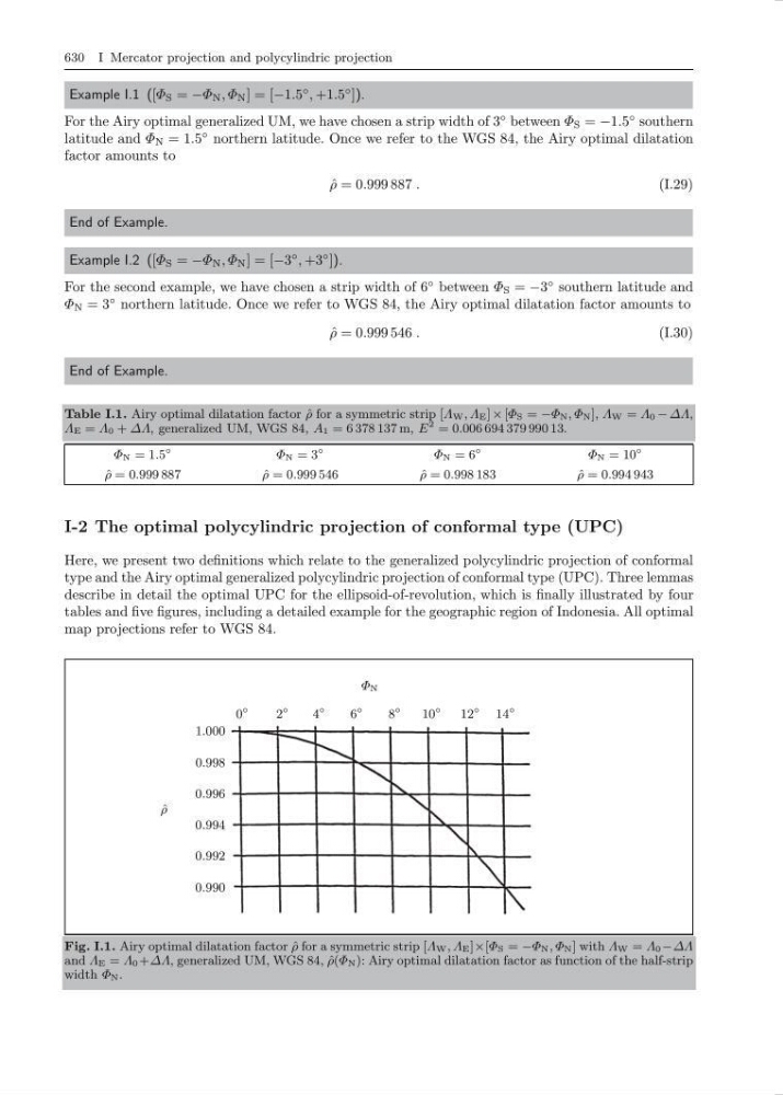
Table I.1. Airy optimal dilatation factor ˆ
ρ for a symmetric strip [Λ W , Λ E ] × [Φ S = −Φ N , Φ N ], Λ W = Λ 0 − ∆Λ,
Λ E = Λ 0 + ∆Λ, generalized UM, WGS 84, A 1 = 6 378 137 m, E
2 = 0.006 694 379 990 13.
Φ N = 1.5
◦
Φ N = 3
◦
Φ N = 6
◦
Φ N = 10
◦
ˆ
ρ = 0.999 887
ˆ
ρ = 0.999 546
ˆ
ρ = 0.998 183
ˆ
ρ = 0.994 943
I-2 The optimal polycylindric projection of conformal type (UPC)
Here, we present two definitions which relate to the generalized polycylindric projection of conformal
type and the Airy optimal generalized polycylindric projection of conformal type (UPC). Three lemmas
describe in detail the optimal UPC for the ellipsoid-of-revolution, which is finally illustrated by four
tables and five figures, including a detailed example for the geographic region of Indonesia. All optimal
map projections refer to WGS 84.
Φ N
ˆ
ρ
0
◦
2
◦
4
◦
6
◦
8
◦
10
◦
12
◦
14
◦
1.000
0.998
0.996
0.994
0.992
0.990
Fig. I.1. Airy optimal dilatation factor ˆ
ρ for a symmetric strip [Λ W , Λ E ]×[Φ S = −Φ N , Φ N ] with Λ W = Λ 0 −∆Λ
and Λ E = Λ 0 +∆Λ, generalized UM, WGS 84, ˆ
ρ(Φ N ): Airy optimal dilatation factor as function of the half-strip
width Φ N .